Calculating Linear or Polynomial Regression in Python

This program performs a linear or polynomial regression on a given dataset and visualizes the result with a graph.

It uses two external Python modules:

• numpy for mathematical operations and calculating the polynomial coefficients.
• matplotlib for generating and displaying the graph.

So, the first step is to import these libraries into the program.

import numpy as np
import matplotlib.pyplot as plt

Next, I define two arrays, `x` and `y`, which represent the observed data (5 pairs of values).

x = np.array([1, 2, 3, 4, 5])
y = np.array([2, 3, 5, 4, 6])

Then, I calculate the polynomial regression using the polyfit(x, y, n) method, where `n` is the degree of the polynomial for the regression curve.

In this case, I choose a third-degree polynomial.

coefficients = np.polyfit(x, y, 3)

The np.polyfit(x, y, 3) function computes the coefficients of a third-degree polynomial (four coefficients) that best fits the data points in \(x\) and \(y\).

Here are the coefficients:

print(coefficients)

array([ 0.16666667, -1.57142857, 5.26190476, -2. ])

After obtaining the coefficients, I use them to define the polynomial function using the poly1d() method.

polynomial = np.poly1d(coefficients)

Then, I generate the predicted values from the polynomial curve for the same \(x\) values.

y_pred_poly = polynomial(x)

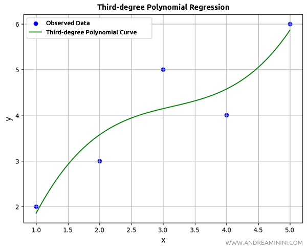
Finally, I display a graph that shows the observed data points as a scatter plot (blue dots) and the third-degree polynomial curve in green.

plt.figure(figsize=(8, 6))
plt.scatter(x, y, color='blue', label='Observed Data') # Observed points
plt.plot(np.linspace(min(x), max(x), 100), polynomial(np.linspace(min(x), max(x), 100)), color='green', label='Third-degree Polynomial Curve')
plt.title("Third-degree Polynomial Regression", fontsize=14)
plt.xlabel("x", fontsize=12)
plt.ylabel("y", fontsize=12)
plt.legend()
plt.grid(True)
plt.show()

This process allows me to visualize the graph of the curve that fits the data points.

The result is a graph that shows how the third-degree polynomial fits the data.

What about linear regression?

Simply change the degree of the polynomial used to fit the data.

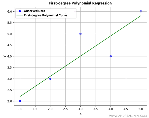
coefficients = np.polyfit(x, y, 1)

In this case, np.polyfit(x, y, 1) calculates the coefficients of a first-degree polynomial (two coefficients) that fits the data points at \(x\) and \(y\) with a regression line.

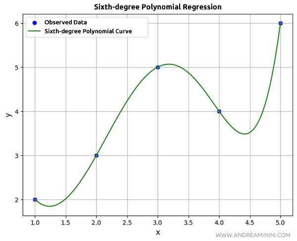
As you increase the degree of the polynomial, the curve fits the points more closely.

For example, if I use a sixth-degree polynomial:

coefficients = np.polyfit(x, y, 6)

The regression curve will pass exactly through the observed data points.

And so on.