Iterative Method for Calculating Square Roots
This algorithm computes an approximate value of the square root of a number N using a transformation function g(x), an initial guess x0, and an iterative loop: $$ x_{n+1} = \frac{1}{2} \cdot \left( x_n + \frac{N}{x_n} \right) $$
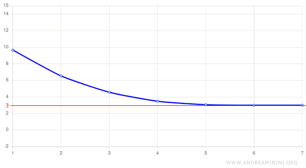
The algorithm converges quadratically to the square root of N.
The process halts when the absolute difference between two successive estimates falls below a user-defined threshold.
For instance, 0.1 or any other value deemed acceptable.
$$ | x_{n+1} - x_n | < 0.1 $$
This threshold controls both the accuracy of the result and the number of iterations required.
The smaller the threshold, the more accurate the estimate-but the more iterations are needed to reach it.
Note. This algorithm is also known as the "Babylonian method" or "Heron’s method." Heron of Alexandria, an ancient Greek mathematician, described the technique in his works, though it was already in use by the Babylonians centuries earlier.
A Practical Example
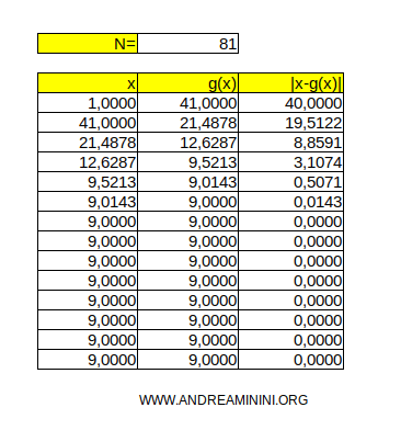
Let’s consider the number N = 81
$$ 81 $$
We’ll compute an estimate of √81 using the iterative approach:
$$ \sqrt{81} $$
We'll set the tolerance to 0.1
$$ | x_{n+1} - x_n | < 0.1 $$
We begin with an initial guess of x0 = 1
$$ x_0 = 1 $$
The choice of x0 is arbitrary-any starting point is valid.
Note. However, when selecting a starting value, it can be helpful to use x0 = N/2 if N is even, or x0 = (N+1)/2 if N is odd. This often reduces the number of iterations compared to starting with x0 = 1.
Now we proceed with the iterative calculation.
Iteration 1
We calculate the next estimate, x1, using the transformation function g(x):
$$ x_1 = \frac{1}{2} \cdot \left( x_0 + \frac{N}{x_0} \right) $$
With N = 81 and x0 = 1:
$$ x_1 = \frac{1}{2} \cdot \left( 1 + \frac{81}{1} \right) $$
$$ x_1 = \frac{1}{2} \cdot 82 $$
$$ x_1 = 41 $$
The first iteration gives us x1 = 41
The difference from the initial guess x0 = 1 is still far too large:
$$ | 41 - 1 | = 40 > 0.1 $$
So we continue with the second iteration.
Iteration 2
Now we compute x2 from x1 = 41:
$$ x_2 = \frac{1}{2} \cdot \left( 41 + \frac{81}{41} \right) $$
$$ x_2 = 21.4878 $$
The difference from x1 is still too large:
$$ | 21.4878 - 41 | = 19.5122 > 0.1 $$
We proceed to the third iteration.
Iteration 3
This time we calculate x3 starting from x2 = 21.4878:
$$ x_3 = \frac{1}{2} \cdot \left( 21.4878 + \frac{81}{21.4878} \right) $$
$$ x_3 = 12.6287 $$
The difference from the previous estimate is smaller, but still above the threshold:
$$ | 12.6287 - 21.4878 | = 8.8591 > 0.1 $$
We move on to the fourth iteration.
Iteration 4
Now we compute x4 from x3 = 12.6287:
$$ x_4 = \frac{1}{2} \cdot \left( 12.6287 + \frac{81}{12.6287} \right) $$
$$ x_4 = 9.5213 $$
The estimate is improving, but the difference is still too large:
$$ | 9.5213 - 12.6287 | = 3.1074 > 0.1 $$
On to iteration five.
Iteration 5
We calculate x5 based on x4 = 9.5213:
$$ x_5 = \frac{1}{2} \cdot \left( 9.5213 + \frac{81}{9.5213} \right) $$
$$ x_5 = 9.0143 $$
Still not close enough:
$$ | 9.0143 - 9.5213 | = 0.4987 > 0.1 $$
We proceed to the sixth and final iteration.
Iteration 6
We compute x6 using x5 = 9.0143:
$$ x_6 = \frac{1}{2} \cdot \left( 9.0143 + \frac{81}{9.0143} \right) $$
$$ x_6 = 9.000011 $$
This time, the difference between x6 and x5 is within the acceptable range:
$$ | 9.000011 - 9.0143 | = 0.014 < 0.1 $$
The algorithm stops here. The final result, x6 = 9.000011, is a close approximation of the square root of 81.
Note. You can improve the accuracy further by lowering the threshold-at the cost of performing more iterations.
Approximating the n-th Root
To approximate the n-th root \( \sqrt[n]{A} \), we can use the generalized version of Newton’s method: \[ x_{k+1} = \frac{1}{n} \cdot \left( (n-1) \cdot x_k + \frac{A}{x_k^{n-1}} \right) \]
Where:
- \( x_k \) is the current estimate
- \( x_{k+1} \) is the updated estimate
- \( A \) is the number whose n-th root we want to compute
- \( n \) is the degree of the root
As with similar iterative methods, the initial guess \( x_0 \) can be chosen freely.
Note. When \( n = 2 \), the formula simplifies to the classic method for computing square roots: \[ x_{k+1} = \frac{1}{2} \cdot \left( (2-1) \cdot x_k + \frac{A}{x_k^{2-1}} \right) \] \[ x_{k+1} = \frac{1}{2} \cdot \left( x_k + \frac{A}{x_k} \right) \]
Example
Let’s compute the cube root of 27:
$$ \sqrt[3]{27} $$
We apply the formula with \( n = 3 \):
\[ x_{k+1} = \frac{1}{3} \left( 2x_k + \frac{27}{x_k^2} \right) \]
We begin with \( x_0 = 1 \). Any non-zero starting value is acceptable; zero must be avoided to prevent division by zero.
We set the convergence threshold to \( S = 0.01 \)
Iteration 1:
\[ x_1 = \frac{1}{3} \left(2 \cdot 1 + \frac{27}{1^2} \right) = \frac{1}{3}(2 + 27) = \frac{29}{3} \approx 9.6667 \]
\[ S_1 = | x_1 - x_0 | = |9.6667 - 1 | = 8.6667 \]
Iteration 2:
\[ x_2 = \frac{1}{3} \left(2 \cdot 9.6667 + \frac{27}{9.6667^2} \right) \approx 6.5408 \]
\[ S_2 = | x_2 - x_1 | = |6.5408 - 9.6667 | = 3.1259 \]
Iteration 3:
\[ x_3 = \frac{1}{3} \left(2 \cdot 6.5408 + \frac{27}{6.5408^2} \right) \approx 4.5709 \]
\[ S_3 = | x_3 - x_2 | = |4.5709 - 6.5408| = 1.9699 \]
Iteration 4:
\[ x_4 = \frac{1}{3} \left(2 \cdot 4.5709 + \frac{27}{4.5709^2} \right) \approx 3.4780 \]
\[ S_4 = | x_4 - x_3 | = |3.4780 - 4.5709| = 1.0929 \]
Iteration 5:
\[ x_5 = \frac{1}{3} \left(2 \cdot 3.4780 + \frac{27}{3.4780^2} \right) \approx 3.0627 \]
\[ S_5 = | x_5 - x_4 | = |3.0627 - 3.4780| = 0.4153 \]
Iteration 6:
\[ x_6 = \frac{1}{3} \left(2 \cdot 3.0627 + \frac{27}{3.0627^2} \right) \approx 3.0013 \]
\[ S_6 = | x_6 - x_5 | = |3.0013 - 3.0627| = 0.0614 \]
Iteration 7:
\[ x_7 = \frac{1}{3} \left(2 \cdot 3.0013 + \frac{27}{3.0013^2} \right) \approx 3.000001 \]
\[ S_7 = | x_7 - x_6 | = |3.000001 - 3.0013| = 0.0012 \]
The stopping condition is now satisfied, since the difference \( S_7 = 0.0012 \) is smaller than the threshold \( S = 0.01 \). The algorithm can terminate.
$$ S_7 = 0.0012 < S = 0.01 $$
After 7 iterations, we obtain a sufficiently accurate approximation: \( x \approx 3.000001 \)
$$ \sqrt[3]{27} \approx 3.000001 $$
In summary, the method converges efficiently and delivers high precision with relatively few iterations.
Note. The exact cube root of 27 is 3, so the algorithm has produced an estimate extremely close to the true value. The more iterations you perform, the greater the accuracy. For this reason, it’s essential to define a stopping criterion at the outset. A typical condition is: $$ | x_k - x_{k-1} | < S $$ This ensures a result within your desired tolerance while avoiding unnecessary computations.
Additional Notes
Further insights into the algorithm:
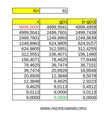
- The initial guess \( x_0 \) can be any non-zero value. For example, even choosing x0 = 1000 or x0 = 9999 would still lead to convergence toward the square root of N = 81. Naturally, the number of iterations required will depend on how close your guess is to the actual root.
- As a rule of thumb, a good starting point is half the value of the radicand: x0 = N/2 if N is even, or x0 = (N+1)/2 if N is odd.
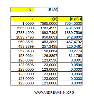
- This method can be used to estimate the square root of any number. For instance, if N = 15129, the algorithm yields its square root-123-within ten iterations.
And so on.


