Definite Integral

The definite integral of a continuous function f(x) over an interval [a,b] is calculated using the following formula: $$ \int_a^b f(x) \:\:dx = F(b) - F(a) $$ This is known as the Fundamental Theorem of Calculus.

The numbers a and b are called the limits of integration.

The function f(x) inside the integral is referred to as the integrand.

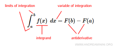
The variable x (dx) is called the variable of integration.

Note. The function F(x) is an antiderivative of f(x), meaning its first derivative is equal to f(x). $$ D[F(x)+k] = f(x) $$ For instance, the function f(x) = 2x has an antiderivative F(x) = x² + k, because its first derivative F'(x) = 2x. The constant k can be any real number, and it vanishes when taking the derivative since D[k] = 0.

What Is the Riemann Definite Integral?

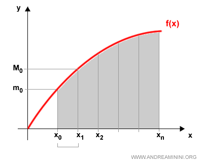
To understand the concept of a definite integral, let's consider a bounded function f(x) defined over a closed interval [a,b] in ℝ.

We divide the interval [a,b] into a partition P consisting of n+1 points:

$$ x_0, x_1, x_2, \ldots, x_n $$

where x₀ is the left endpoint a, and x_n is the right endpoint b of the interval.

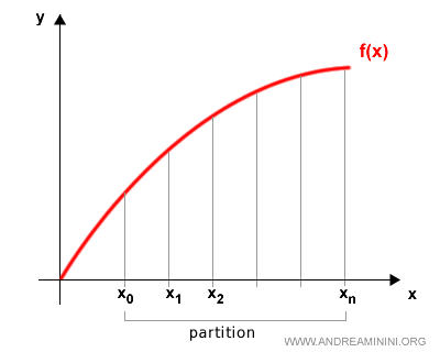
This partition P defines n subintervals:

$$ [x_{k-1}, x_k] \:\:\: \text{for} \:\: k = 1, \ldots, n $$

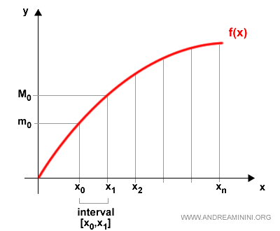
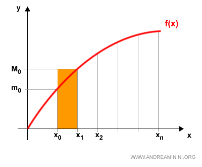
Each subinterval is associated with a minimum and a maximum value of the function:

$$ m_k = \inf \{ f(x) : x \in [x_{k-1}, x_k] \} $$

$$ M_k = \sup \{ f(x) : x \in [x_{k-1}, x_k] \} $$

For example, the first subinterval [x₀, x₁] has a minimum value m₀ and a maximum value M₀.

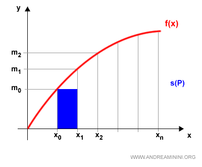
Multiplying the minimum value m_k by the width of its corresponding interval [x_k-1, x_k] gives the area of a rectangle inscribed under the graph of the function:

$$ m_k \cdot (x_k - x_{k-1}) $$

For instance, in the first interval, this gives a rectangle with height m₀ and base [x₀, x₁].

The same applies to the maximum values M_k:

$$ M_k \cdot (x_k - x_{k-1}) $$

For example, in the first interval, the resulting rectangle has height M₀ and the same base.

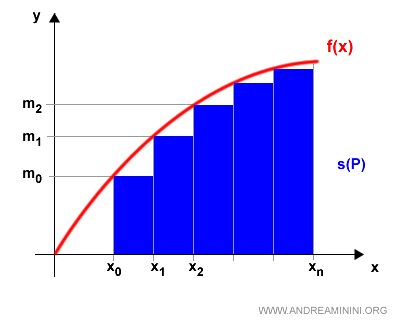
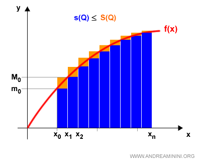
The sum of the areas of all the inscribed rectangles is called the lower Riemann sum:

$$ s(P) = \sum_{k=1}^{n} m_k \cdot (x_k - x_{k-1}) $$

Here’s how it looks graphically:

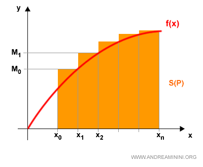
The sum of the circumscribed rectangles is called the upper Riemann sum:

$$ S(P) = \sum_{k=1}^{n} M_k \cdot (x_k - x_{k-1}) $$

Here’s the corresponding graph:

By definition, the minimum m_k is always less than or equal to the maximum M_k:

$$ m_k \le M_k $$

Therefore, the lower sum s(P) is always less than or equal to the upper sum S(P):

$$ s(P) \le S(P) $$

Geometrically, the upper sum always exceeds the lower sum:

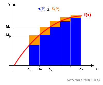
It’s easy to see that the actual area under the curve f(x) lies somewhere between s(P) and S(P):

If we refine the partition by using a different one, say Q, we get new upper and lower sums:

$$ s(Q) \\ S(Q) $$

This new partition Q consists of more subintervals.

As a result, the difference between the upper and lower sums becomes smaller than it was for P.

Note. Visually, the difference S(Q) - s(Q) corresponds to the orange area exceeding the blue one. As you can see, this orange area is much smaller than the difference S(P) - s(P) for the earlier partition. Of course, we could create infinitely many other partitions beyond just P and Q. The more intervals a partition has, the smaller the gap between the upper and lower sums becomes.

Let’s now define set A to include all lower sums from every possible partition (e.g., P, Q, etc.):

$$ A = \{s(P), s(Q) \} $$

And set B to include all the corresponding upper sums:

$$ B = \{S(P), S(Q) \} $$

These two sets are disjoint.

If there exists a unique value c that separates sets A and B, then the function f(x) is said to be Riemann integrable over [a,b]. $$ c = \sup A = \inf B $$ This value c is called the definite integral of f(x) over [a,b] and is denoted by the symbol: $$ \int_a^b f(x) \:\: dx $$

A Practical Example

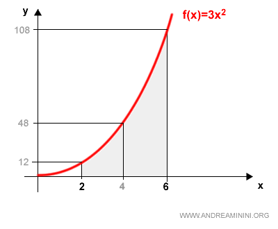
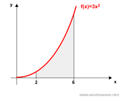
Let’s take a look at the function:

$$ f(x) = 3x^2 $$

Here’s its graph:

To determine the area under the curve from x = 2 to x = 6, we compute the definite integral:

$$ \int_2^6 3x^2 \: dx $$

We begin by partitioning the interval using a division, P, that splits it into two equal subintervals.

This creates two inscribed and two circumscribed rectangles.

Starting with the inscribed rectangles:

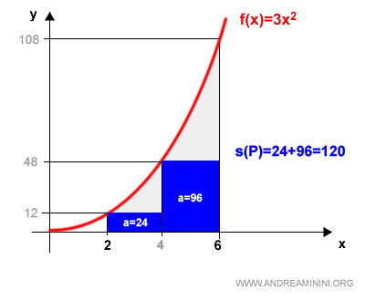
The first rectangle has an area of 24, and the second 96.

So, the lower sum for partition P is:

$$ s(P) = 24 + 96 = 120 $$

Now let’s look at the circumscribed rectangles for the same partition:

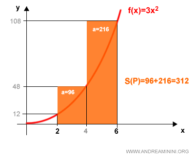
The first rectangle has an area of 96, and the second 216.

Hence, the upper sum is:

$$ S(P) = 96 + 216 = 312 $$

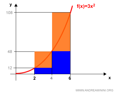
It’s clear that the actual area under the curve lies between these two values:

$$ s(P) \leq \text{Area} \leq S(P) $$

That is:

$$ 120 \leq \text{Area} \leq 312 $$

Graphically, this area lies between the inscribed and circumscribed rectangles:

To improve the estimate, we can use a finer partition, Q, this time dividing the interval [2, 6] into four subintervals.

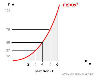
This gives four inscribed and four circumscribed rectangles.

Let’s examine the inscribed rectangles first:

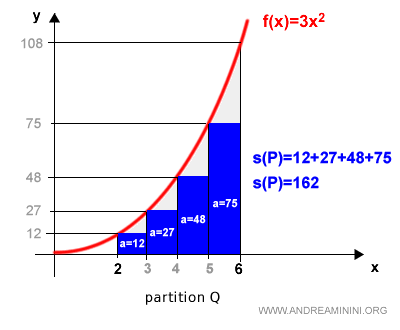
The lower sum for Q is:

$$ s(Q) = 162 $$

And now the circumscribed rectangles:

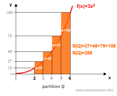
The upper sum for Q is:

$$ S(Q) = 258 $$

Now we have the lower and upper sums for both partitions P and Q:

$$ s(P) = 120 \\ S(P) = 312 \\ s(Q) = 162 \\ S(Q) = 258 $$

We can collect the lower sums into a set A:

$$ A = \{ s(P), s(Q) \} = \{ 120, 162 \} $$

And the upper sums into a set B:

$$ B = \{ S(P), S(Q) \} = \{ 312, 258 \} $$

The least upper bound of set A is 162, and the greatest lower bound of set B is 258:

$$ \sup(A) = 162 \\ \inf(B) = 258 $$

According to Riemann’s definition, the exact area under the curve lies somewhere between these two bounds:

$$ \sup(A) \leq \text{Area} \leq \inf(B) $$

So we get:

$$ 162 \leq \text{Area} \leq 258 $$

As we keep refining the partition - dividing the interval into increasingly smaller segments - the lower and upper sums converge toward the actual area.

Once the values of sup(A) and inf(B) meet, we have precisely determined the value of the definite integral: the exact area under the curve.

The Fundamental Theorem of Calculus

Fortunately, we usually don’t need to rely on Riemann sums to compute a definite integral. There’s a more powerful and efficient method.

It’s called the Fundamental Theorem of Calculus.

$$ \int_a^b f(x) \:\:dx = F(b) - F(a) $$

This theorem allows us to evaluate a definite integral by simply finding an antiderivative of the integrand.

Once we have an antiderivative F(x) of f(x), calculating the integral becomes straightforward and exact.

Note. It’s important to keep in mind that the function must be continuous and differentiable, and in some cases, finding an antiderivative can be quite challenging.

Example

Let’s revisit our previous function and apply the Fundamental Theorem:

$$ \int_2^6 3x^2 \:\: dx $$

An antiderivative of f(x) is:

$$ F(x) = x^3 $$

Since its first derivative is:

$$ D[x^3] = 3x^2 $$

The definite integral then evaluates to:

$$ \int_2^6 3x^2 \:\: dx = F(6) - F(2) = 6^3 - 2^3 = 208 $$

This gives us the exact area under the curve from x = 2 to x = 6 - no approximation needed.

And that’s how the Fundamental Theorem streamlines the process of calculating definite integrals.