Triple Integrals

A triple integral extends the idea of a double integral to functions of three variables, \( f(x, y, z) \), over a solid region \( E \subseteq \mathbb{R}^3 \). It is written as: \[\iiint_E f(x, y, z)\, dV\] Here, \( dV \) represents an infinitesimal volume element (e.g., \( dx\,dy\,dz \)), and \( E \) is a three-dimensional region in space.

At first glance, the geometric and physical interpretation of a triple integral can be hard to visualize.

Simply put, if \( f(x, y, z) \geq 0 \), the triple integral gives the total amount of some quantity - such as mass, energy, or electric charge - distributed in space according to the density function \( f \):

$$ \iiint_E f(x, y, z)\, dV $$

If \( f(x, y, z) \) takes on both positive and negative values, the integral instead measures the net contribution - the difference between what the function adds to the volume and what it subtracts:

$$ \iiint_E f(x, y, z)\, dV = \text{positive part} - \text{negative part} $$

For instance, if \( f(x, y, z) \) models a density, then regions where \( f > 0 \) add material (positive mass), while regions where \( f < 0 \) remove it (a deficit, or negative mass). The integral thus represents the overall balance between what’s present and what’s lacking. In physics or engineering, a sign-changing function might describe opposing flows - e.g., inflow versus outflow.

How is it computed?

A triple integral is typically evaluated as an iterated integral, using an order of integration that reflects the geometry of the region:

\[ \iiint_E f(x, y, z)\, dV = \int_{x_0}^{x_1} \int_{y_0(x)}^{y_1(x)} \int_{z_0(x,y)}^{z_1(x,y)} f(x, y, z)\, dz\,dy\,dx \]

The order can be rearranged (e.g., \( dz\,dx\,dy \), etc.) depending on the shape of the domain \( E \).

While changing the order of integration doesn’t affect the value of the integral, the limits must be carefully redefined to correctly describe the region in the new variable order.

A Practical Example

Let’s compute the triple integral of the function \[ f(x, y, z) = z \] over the cube \[ E = [0,1] \times [0,1] \times [0,1] \]

In this case, the function \( f(x, y, z) = z \) models a density that increases with height.

The integral tells us the total amount (e.g., total mass) present in the cube, assuming a density that varies linearly with \( z \).

We express the integral in iterated form:

\[ \iiint_E z\, dV = \int_0^1 \int_0^1 \int_0^1 z\, dz\,dy\,dx \]

First, integrate with respect to \( z \):

\[ \int_0^1 z\, dz = \left[ \frac{z^2}{2} \right]_0^1 = \frac{1}{2} \]

Then with respect to \( y \):

\[ \int_0^1 \frac{1}{2}\, dy = \frac{1}{2} \]

And finally with respect to \( x \):

\[ \int_0^1 \frac{1}{2}\, dx = \frac{1}{2} \]

So, the value of the triple integral is:

\[ \iiint_E z\, dV = \frac{1}{2} \]

This means the total mass in the cube is \( \frac{1}{2} \) units. Since the density increases linearly from zero at the base (\( z = 0 \)) to one at the top (\( z = 1 \)), the result corresponds to the average value of \( z \) times the volume of the cube.

The average of \( z \) over the unit cube is \( \frac{1}{2} \), and since the volume is \( 1 \), the integral returns \( \frac{1}{2} \times 1 = \frac{1}{2} \).

Example 2

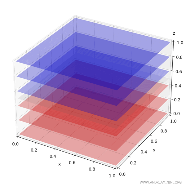
Now consider the function \( f(x, y, z) = z - 0.5 \), again over the unit cube \( E = [0,1]^3 \). This function is negative below the plane \( z = 0.5 \) and positive above it.

The triple integral becomes:

\[ \iiint_E (z - 0.5)\, dV = \int_0^1 \int_0^1 \int_0^1 (z - 0.5)\, dz\,dy\,dx \]

We begin with the innermost integral:

\[ \int_0^1 (z - 0.5)\, dz = \left[ \frac{z^2}{2} - 0.5z \right]_0^1 = \left( \frac{1}{2} - 0.5 \right) = 0 \]

Since the result is zero, the remaining two integrals are also zero:

\[ \int_0^1 \int_0^1 0\, dy\,dx = 0 \]

So the value of the triple integral is:

\[ \iiint_E (z - 0.5)\, dV = 0 \]

This outcome reflects the symmetry of the function \( z - 0.5 \): it contributes negative values below \( z = 0.5 \) and equal positive values above it. The two regions cancel out perfectly.

This 3D plot of \( f(x, y, z) = z - 0.5 \) over the cube \( [0,1]^3 \) highlights:

• Blue layers: where the function is positive (above \( z = 0.5 \))
• Red layers: where the function is negative (below \( z = 0.5 \))

Because the function is perfectly symmetric about the plane \( z = 0.5 \), the positive and negative contributions cancel each other exactly, yielding a net integral of zero.

Note. From a physical perspective, this could represent equal and opposite forces - e.g., a push and a pull - that balance each other out.

And so on.