Gradient

The gradient of a scalar function or field f(x, y, z) is a vector field whose components are the partial derivatives of f with respect to the Cartesian coordinates (x, y, z). $$ \nabla f = \frac{ \partial f}{\partial x} \vec{u}_x + \frac{ \partial f}{\partial y} \vec{u}_y + \frac{ \partial f}{\partial z} \vec{u}_z $$ This differential operator, denoted by the nabla symbol ∇ (an inverted triangle), is also commonly written as grad: $$ \text{grad} \, f = \frac{ \partial f}{ \partial x} \vec{u}_x + \frac{ \partial f}{ \partial y} \vec{u}_y + \frac{ \partial f}{ \partial z} \vec{u}_z $$

Here, u_x, u_y, and u_z are the unit vectors along the x-, y-, and z-axes of three-dimensional space.

The scalar field f(x, y, z) is a real-valued function.

The gradient ∇f, by contrast, is a vector-valued function.

What does the gradient represent?

The gradient maps a scalar field to a vector field. It captures both the rate and direction of the steepest increase in the scalar quantity.

For instance, the temperature gradient indicates how and in which direction the temperature changes most rapidly in space.

Note. The gradient points in the direction of maximum increase of the scalar field f(x, y, z). Its magnitude corresponds to the steepest rate of change at that point.

Key Properties of the Gradient

Given a gradient ∇f and a vector v, the dot product ∇f · v gives the directional derivative of f in the direction of v:

$$ \nabla f \cdot \vec{v} = D_v f $$

What is a directional derivative? The directional derivative measures how a function f(x, y, z) changes as you move in a specific direction, defined by the vector v: $$ D_v f = \lim_{h \to 0} \frac{f(x+h \cdot \vec{v}, \ y+h \cdot \vec{v}, \ z+h \cdot \vec{v}) - f(x, y, z)}{h} $$ It generalizes the concept of partial derivatives, which measure change only along the coordinate axes: $$ D_x f = \lim_{\Delta x \to 0} \frac{f(x+\Delta x, y, z) - f(x, y, z)}{\Delta x} $$

If we consider an infinitesimal displacement in the direction of the position vector v (position vector):

$$ d \vec{v} = dx \cdot \vec{u}_x + dy \cdot \vec{u}_y + dz \cdot \vec{u}_z $$

The directional derivative of f in this direction is given by the gradient:

$$ \frac{d \ f(\vec{v})}{d \ \vec{v}} = \nabla f $$

Thus, the differential of the function in the direction of v is:

$$ df(\vec{v}) = \nabla f \cdot d \vec{v} $$

And therefore, the function value at a nearby point becomes:

$$ f(\vec{v} + d \vec{v}) = f(\vec{v}) + df(\vec{v}) = f(\vec{v}) + \nabla f(\vec{v}) \cdot \vec{v} $$

A Concrete Example

Let’s take a function of two variables:

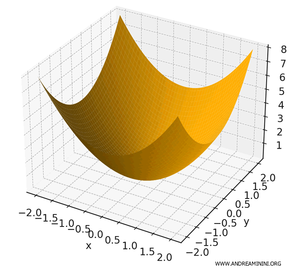
\[ f(x, y) = x^2 + y^2 \]

This function assigns to each point \( (x, y) \) the square of its distance from the origin.

To compute the gradient \( \nabla f \), we calculate the partial derivatives with respect to \( x \) and \( y \):

\[ \frac{\partial f}{\partial x} = 2x \]

\[ \frac{\partial f}{\partial y} = 2y \]

Therefore, the gradient is:

\[ \nabla f(x, y) = 2x \, \vec{u}_x + 2y \, \vec{u}_y \]

In vector notation:

\[ \nabla f(x, y) = \begin{pmatrix} 2x \\ 2y \end{pmatrix} \]

The gradient vectors point directly away from the origin. This reflects the fact that the function \( f(x, y) = x^2 + y^2 \) increases most rapidly in the radial direction.

The magnitude of the gradient is \( |\nabla f| = \sqrt{(2x)^2 + (2y)^2} = 2\sqrt{x^2 + y^2} \), representing the rate at which the function increases as you move away from the origin.

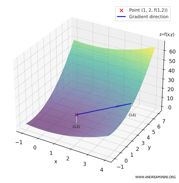
For example, at the point \( (1, 2) \):

\[ \nabla f(1, 2) = \begin{pmatrix} 2 \cdot 1 \\ 2 \cdot 2 \end{pmatrix} = \begin{pmatrix} 2 \\ 4 \end{pmatrix} \]

This means that at \( (1, 2) \), the function increases most rapidly in the direction of the vector \( (2, 4) \), pointing toward the point \( (3, 6) \).

You can repeat this process at any point in the (x, y) plane.

The result is the gradient vector field for the function \( f(x, y) = x^2 + y^2 \):

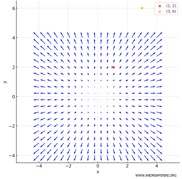
Each arrow represents the **gradient vector** at a given point \( (x, y) \).

All vectors point outward - away from the origin - because the function increases with distance from the center.

The points \( (1, 2) \) and \( (3, 6) \) are marked in red and orange, respectively.

You can also add contour lines to show level curves - sets of points where the function takes on the same value \( f(x, y) = c \).

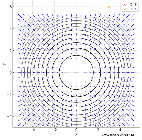
In this case, the contour lines are concentric circles, since \( f(x, y) = x^2 + y^2 \).

The Gradient Points in the Direction of Greatest Increase

The gradient \( \nabla f(x_0) \) is a vector that indicates the direction in which the function increases most rapidly.

Put simply, the gradient indicates the direction of steepest ascent - that is, the path along which the function increases at the fastest rate.

The magnitude of the gradient quantifies the rate of increase in that direction.

Conversely, the direction of steepest descent is given by the negative gradient vector.

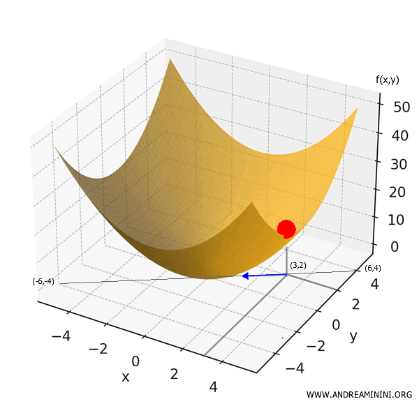
Example

Consider the function:

$$ f(x,y) = x^2 + y^2 $$

This is the equation of a bowl-shaped surface - a familiar example we've seen earlier.

Suppose we drop a ball at the point (3,2). Which direction will it start to roll?

To find out, we begin by computing the partial derivatives of the function with respect to \( x \) and \( y \):

$$ f_x = 2x $$

$$ f_y = 2y $$

These expressions allow us to construct the gradient vector of the function:

$$ \nabla f(x,y) = (2x, 2y) $$

Evaluating the gradient at the point (3,2) gives:

$$ \nabla f(3,2) = (2 \cdot 3, 2 \cdot 2) = (6, 4) $$

The gradient vector always points in the direction of steepest increase - that is, the direction in which the function rises most rapidly.

However, since the ball is influenced by gravity, it rolls downhill - in the direction where the function decreases most rapidly. This direction is exactly opposite to the gradient:

$$ -\nabla f(3,2) = (-6, -4) $$

Therefore, the ball will move in the direction of the vector \( (-6, -4) \).

Note. We can also normalize this direction vector to obtain a unit vector that points in the same direction: \[ \mathbf{u} = \frac{-\nabla f(3,2)}{\lVert \nabla f(3,2) \rVert} = \frac{(-6, -4)}{\sqrt{6^2 + 4^2}} = \Bigl(-\tfrac{3}{\sqrt{13}},\, -\tfrac{2}{\sqrt{13}}\Bigr) \] Dividing by the magnitude of the gradient gives us a vector with unit length, which is useful for describing direction independently of speed or steepness. The geometric and physical interpretation remains the same.

Proof

To demonstrate this, we start with the definition of the directional derivative of a function \( f \) at the point \( x_0 \) in the direction of a vector \( \vec{v} \).

The directional derivative is given by the dot product of the gradient of \( f \) at \( x_0 \) and the direction vector \( \vec{v} \):

\[ \frac{\partial f}{\partial \vec{v}}(\vec{x}_0) = \nabla f(x_0) \cdot \vec{v} \]

Using the geometric definition of the dot product, this expression can be rewritten as:

\[ \frac{\partial f}{\partial \vec{v}}(x_0) = |\nabla f(x_0)| \cdot |\vec{v}| \cdot \cos\theta \]

Here, \( \theta \) is the angle between the gradient \( \nabla f(x_0) \) and the direction vector \( \vec{v} \).

This formula shows that the value of the directional derivative depends on three key elements:

1. The magnitude of the gradient, which reflects how sharply the function is changing overall;
2. The length of the direction vector \( \vec{v} \), which is typically normalized so that \( |\vec{v}| = 1 \);
3. The cosine of the angle between the gradient and the direction vector.

Since the magnitude of the gradient is independent of the direction chosen, and the direction vector is usually unit-length, the directional derivative primarily varies with the cosine of the angle \( \theta \).

Let’s analyze how the cosine affects the directional derivative for different values of \( \theta \):

• If \( \theta = 0^\circ \), then \( \cos\theta = 1 \): the vectors are aligned and point in the same direction. In this case, the directional derivative attains its maximum value, and the direction coincides with that of the gradient.
• If \( \theta = 180^\circ \), then \( \cos\theta = -1 \): the vectors are parallel but point in opposite directions. The directional derivative reaches its minimum in this case, pointing in the direction opposite to the gradient.
• If \( \theta = 90^\circ \), then \( \cos\theta = 0 \): the vectors are orthogonal. The directional derivative is zero, meaning the function does not vary in that direction.

This analysis confirms that the gradient \( \nabla f(x_0) \) not only identifies the direction of steepest ascent, but its magnitude also represents the maximum rate of increase of the function at that point.

Relationship Between the Gradient and Level Curves

The gradient is always perpendicular to level curves.

This means that if you draw a level curve - such as a circle - the gradient at any point along the curve is a vector that is orthogonal to the curve and points radially outward from it.

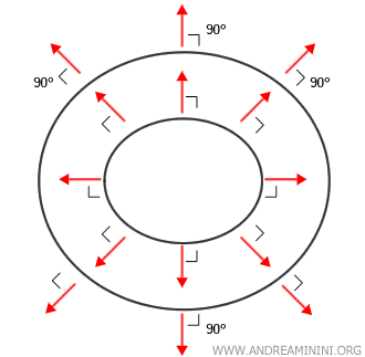
Level curves represent the set of points where a function takes on a constant value, that is, $ f(x,y) = c $.

In contrast, the gradient points in the direction of steepest ascent: $ \nabla f(x, y) = \left( \frac{\partial f}{\partial x}, \frac{\partial f}{\partial y} \right) $.

So, if the function remains constant in one direction (along a level curve) and increases most rapidly in another (along the gradient), those directions must be perpendicular - they form a right angle.

Example

The gradient of the function $ f(x,y) = x^2 + y^2 $ defines a vector field, assigning to each point in the plane a vector pointing in the direction of greatest increase, and in the opposite direction, the steepest decrease.

As shown, the gradient vector at any point $ (x,y,z) $ on the surface defined by $ z = f(x,y) $ is perpendicular to the level curve passing through that point.

The only point where the gradient is zero is at the origin, $ (x,y,z) = (0,0,0) $, the center of the level curves for this function - there, the vector has no direction.

Note. A vanishing gradient indicates a critical point - where the function does not increase or decrease in any direction. In such cases, it's useful to compute the Laplacian, which is the sum of the second partial derivatives with respect to all spatial variables: \[\Delta f = \frac{\partial^2 f}{\partial x^2} + \frac{\partial^2 f}{\partial y^2}\] The Laplacian at that point helps classify the nature of the critical point: if \( \Delta f > 0 \), it’s a local minimum; if \( \Delta f < 0 \), a local maximum; and if \( \Delta f = 0 \), the behavior is inconclusive and requires further analysis.

Proof

Let \( (x_0, y_0) \) be a point in the domain of \( f \), and consider a smooth curve \( \gamma(t) = (x(t), y(t)) \) that lies entirely on a level curve of \( f \).

Since the value of the function remains constant along this curve, its directional derivative must vanish:

\[ f(x(t), y(t)) = \text{constant} \quad \Rightarrow \quad \frac{d}{dt} f(x(t), y(t)) = 0 \]

Applying the chain rule yields:

\[ \frac{d}{dt} f(x(t), y(t)) = \frac{\partial f}{\partial x} \cdot \frac{dx}{dt} + \frac{\partial f}{\partial y} \cdot \frac{dy}{dt} = \nabla f \cdot \vec{v} = 0 \]

Here, \( \vec{v} = \left( \frac{dx}{dt}, \frac{dy}{dt} \right) \) is the tangent vector to the curve \( \gamma(t) \).

Since the dot product \( \nabla f \cdot \vec{v} = 0 \), the gradient \( \nabla f \) is orthogonal to the tangent vector - that is, it is perpendicular to the level curve.

And so on.