Quartiles

What are quartiles?

Quartiles are three positional values (quantiles) that divide a data set into four equal parts.

Each part contains an equal number of elements.

There are three quartiles:

• The first quartile (Q₁) represents the first 1/4 of the data set (25%).
• The second quartile (Q₂) represents the first 2/4 of the data set (50%).
• The third quartile (Q₃) represents the first 3/4 of the data set (75%).

Example: In this series, the first quartile Q₁=4.5, the second quartile Q₂=6.5, and the third quartile Q₃=8.5 divide the distribution into four parts: $$ X = \{ \underbrace{3,4}, \color{red}{Q_1}, \underbrace{5, 6}, \color{red}{ Q_2 }, \underbrace{7, 8}, \color{red}{Q_3}, \underbrace{9, 10} \} $$. Sometimes, the term "quartile zero" (Q₀) is used to refer to the first element of the ordered distribution (e.g., 3), and "quartile four" (Q₄) to refer to the last element (e.g., 11).

How to calculate quartiles

There are two main methods for calculating quartiles, depending on whether you're working with a simple data series or a frequency distribution.

Series

To calculate the quartiles of a data series:

1. Sort the data in ascending order.
2. Multiply the number of elements in the series by p=1/4 for Q₁, p=2/4 for Q₂, and p=3/4 for Q₃: $$ k = n \cdot p $$
3. Determine the position of the quartile:
   • If k is an integer, the quartile is the average of the k-th and (k+1)-th elements in the data set.
   • If k is not an integer, round up to the next whole number to find the position of the quartile.

Frequency distributions

To calculate quartiles in a frequency distribution:

• Calculate the cumulative absolute frequencies for each class in the distribution.
• Divide the total cumulative frequency by 1/4, 2/4, and 3/4 to find the positions of Q₁, Q₂, and Q₃ within the cumulative frequencies.
• Identify the frequency intervals that contain Q₁, Q₂, and Q₃. These intervals correspond to the quartiles.

Note: There are several methods for calculating quartiles. For example, some use linear interpolation to estimate the value of the quartile within a class, while others approximate it to the midpoint of the class.

A practical example

Example 1

This data set contains n=9 elements:

$$ X = \{ 9,6,11,8,4,7,10,3,5 \} $$

First, sort the data in ascending order:

$$ X = \{ 3,4,5,6,7,8,9,10,11 \} $$

To calculate the first quartile (Q₁), multiply the number of elements (n=9) by 1/4:

$$ k = n \cdot \frac{1}{4} = 9 \cdot \frac{1}{4} = 2.25 $$

Since the result is a decimal, round up to the next whole number (k=3) to find the position of Q₁.

$$ X = \{ 3,4,\color{red}{5},6,7,8,9,10,11 \} $$

The third element (k=3) is 5.

$$ Q_1 = 5 $$

Therefore, the first quartile of this data set is Q₁=5.

$$ X = \{ 3,4,\underbrace{5}_{Q_1},6,7,8,9,10,11 \} $$

To calculate the second quartile (Q₂), multiply the number of elements (n=9) by 2/4:

$$ k = n \cdot \frac{2}{4} = 9 \cdot \frac{2}{4} = 4.5 $$

Since the result is a decimal, round up to the next whole number (k=5) to find the position of Q₂.

$$ X = \{ 3,4,5,6,\color{red}{7},8,9,10,11 \} $$

The fifth element (k=5) is 7.

$$ Q_2 = 7 $$

Therefore, the second quartile of this data set is Q₂=7.

$$ X = \{ 3,4,5,6,\underbrace{7}_{Q_2},8,9,10,11 \} $$

To calculate the third quartile (Q₃), multiply the number of elements (n=9) by 3/4:

$$ k = n \cdot \frac{3}{4} = 9 \cdot \frac{3}{4} = 6.75 $$

Since the result is a decimal, round up to the next whole number (k=7) to find the position of Q₃.

$$ X = \{ 3,4,5,6,7,8,\color{red}{9},10,11 \} $$

The seventh element (k=7) is 9.

$$ Q_3 = 9 $$

Therefore, the third quartile of this data set is Q₃=9.

$$ X = \{ 3,4,5,6,7,8,\underbrace{9}_{Q_3},10,11 \} $$

In summary, the three quartiles Q₁ = 5, Q₂ = 7, and Q₃ = 9 divide the data into four parts:

$$ X = \{ \underbrace{3,4}, \underset{Q_1}{\color{red}5}, \underbrace{6}, \underset{Q_2}{\color{red}7}, \underbrace{8}, \underset{Q_3}{\color{red}9}, \underbrace{10,11} \} $$

Note: In this case, the three quartiles are approximate values that belong to the data set X.

Example 2

Now let's look at the same data set with one element removed.

This time, the data set contains n=8 elements:

$$ X = \{ 9,6,8,4,7,10,3,5 \} $$

Sort the data in ascending order:

$$ X = \{ 3,4,5,6,7,8,9,10 \} $$

To calculate the first quartile (Q₁), multiply the number of elements (n=8) by 1/4:

$$ k = n \cdot \frac{1}{4} = 8 \cdot \frac{1}{4} = 2 $$

Since k=2 is an integer, take the average of the values at positions k=2 and k+1=3.

$$ X = \{ 3,\color{red}4,\color{red}5,6,7,8,9,10 \} $$

The second element (k=2) is 4, and the third element (k=3) is 5.

Therefore, the first quartile of this data set is Q₁=4.5.

$$ Q_1 = \frac{4+5}{2} = 4.5 $$

To calculate the second quartile (Q₂), multiply the number of elements (n=8) by 2/4:

$$ k = n \cdot \frac{2}{4} = 8 \cdot \frac{2}{4} = 4 $$

Since k=4 is an integer, take the average of the values at positions k=4 and k+1=5.

$$ X = \{ 3,4,5,\color{red}6,\color{red}7,8,9,10 \} $$

The fourth element (k=4) is 6, and the fifth element (k=5) is 7.

Therefore, the second quartile of this data set is Q₂=6.5.

$$ Q_2 = \frac{6+7}{2} = 6.5 $$

To calculate the third quartile (Q₃), multiply the number of elements (n=8) by 3/4:

$$ k = n \cdot \frac{3}{4} = 8 \cdot \frac{3}{4} = 6 $$

Since k=6 is an integer, take the average of the values at positions k=6 and k+1=7.

$$ X = \{ 3,4,5,6,7,\color{red}8,\color{red}9,10 \} $$

The sixth element (k=6) is 8, and the seventh element (k=7) is 9.

Therefore, the third quartile of this data set is Q₃=8.5.

$$ Q_3 = \frac{8+9}{2} = 8.5 $$

In summary, the three quartiles Q₁ = 4.5, Q₂ = 6.5, and Q₃ = 8.5 divide the data into four parts:

$$ X = \{ \underbrace{3,4}, \color{red}{Q_1}, \underbrace{5, 6}, \color{red}{ Q_2 }, \underbrace{7, 8}, \color{red}{Q_3}, \underbrace{9, 10} \} $$

Note: In this case, the three quartiles are approximate values that do not belong to the data set X.

Example 3

Let's consider this frequency distribution:

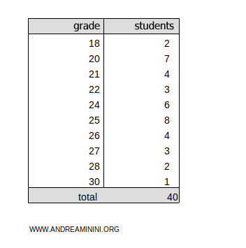
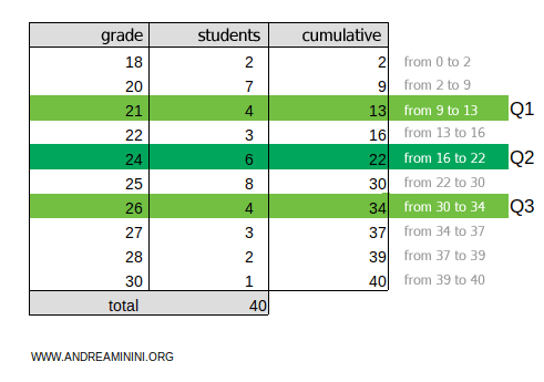
This represents the grades of 40 students. The grades range from 18 to 30, and the frequencies represent how many students achieved each grade.

To find the quartiles, add a column for the cumulative frequencies, starting with the first class.

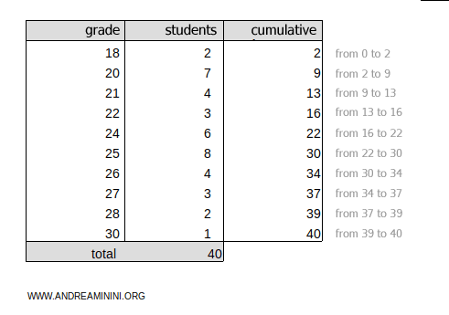
The total cumulative frequency is f_tot=40.

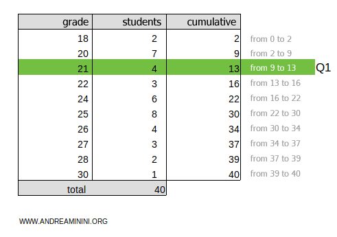
To calculate the first quartile, multiply the total cumulative frequency f_tot=40 by 1/4:

$$ k =f_{tot} \cdot \frac{1}{4} = 40 \cdot \frac{1}{4} = 10 $$

The result, 10, lies in the cumulative frequency range 9-13.

Therefore, the first quartile is in the class Q₁=21.

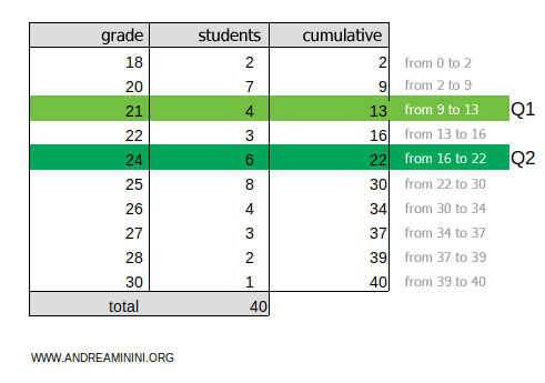
To calculate the second quartile, multiply the total cumulative frequency f_tot=40 by 2/4:

$$ k =f_{tot} \cdot \frac{2}{4} = 40 \cdot \frac{2}{4} = 20 $$

The result, 20, lies in the cumulative frequency range 16-22.

Therefore, the second quartile is in the class Q₂=24.

To calculate the third quartile, multiply the total cumulative frequency f_tot=40 by 3/4:

$$ k =f_{tot} \cdot \frac{3}{4} = 40 \cdot \frac{3}{4} = 30 $$

The result, 30, lies in the cumulative frequency range 30-34.

Therefore, the third quartile is in the class Q₃=26.

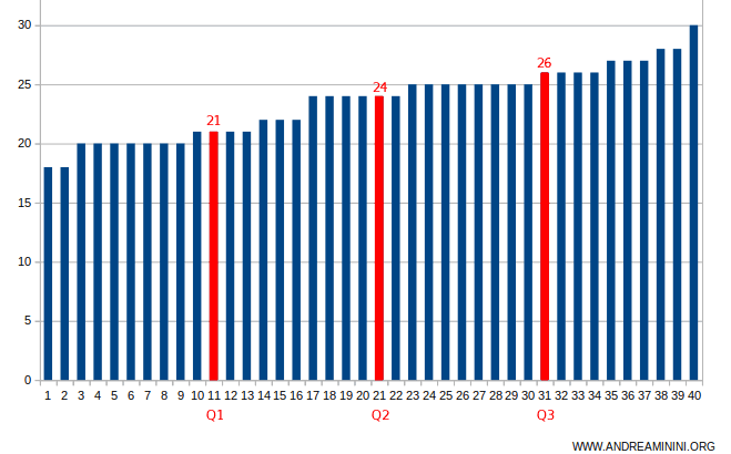
Note: When listing the 40 grades in order from lowest to highest, the three quartiles Q₁, Q₂, and Q₃ divide the series into four equal parts.

Example 4

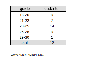
This frequency distribution is divided into classes:

Next, add a column for the cumulative absolute frequencies:

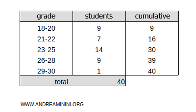
The total cumulative frequency is f_tot=40.

To find the first quartile (Q₁), multiply the total cumulative frequency f_tot=40 by 1/4:

$$ k =f_{tot} \cdot \frac{1}{4} = 40 \cdot \frac{1}{4} = 10 $$

The result, 10, lies within the cumulative frequency range 9-16 for the class 21-22.

In this case, linear interpolation is used to find a more precise quartile value:

$$ Q_1 = x_{inf} + (x_{sup} - x_{inf}) \cdot \frac{c - n_{prec}}{n_{classe}} $$

Here’s what the terms mean:

• x_inf=21 and x_sup=22 are the boundaries of the class 21-22.
• c=10 is the position of the first quartile.
• n_classe=7 is the frequency of the class 21-22.
• n_prec=9 is the cumulative frequency of the classes preceding 21-22.

Substitute the values and calculate:

$$ Q_1 = 21 + (22 - 21 ) \cdot \frac{10 - 9}{7} $$

$$ Q_1 = 21 + 1 \cdot \frac{1}{7} $$

$$ Q_1 = 21.14 $$

Therefore, the first quartile is Q₁=21.14.

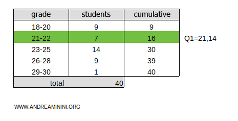
Note: Alternatively, you can approximate the first quartile by calculating the midpoint of the class. In this case, the midpoint of the class 21-22 is 21.5, giving an approximate first quartile of Q₁=21.5. This method is quicker but less precise than linear interpolation.

To calculate the second quartile (Q₂), multiply the total cumulative frequency f_tot=40 by 2/4:

$$ k =f_{tot} \cdot \frac{2}{4} = 40 \cdot \frac{2}{4} = 20 $$

The result, 20, lies within the cumulative frequency range 16-30 for the class 23-25.

Again, we use linear interpolation to find the precise value of the second quartile:

$$ Q_2 = x_{inf} + (x_{sup} - x_{inf}) \cdot \frac{c - n_{prec}}{n_{classe}} $$

Here’s what the terms mean:

• x_inf=23 and x_sup=25 are the boundaries of the class 23-25.
• c=20 is the position of the second quartile.
• n_classe=14 is the frequency of the class 23-25.
• n_prec=16 is the cumulative frequency of the classes preceding 23-25.

Substitute the values and calculate:

$$ Q_2 = 23 + (25 - 23) \cdot \frac{20 - 16}{14} $$

$$ Q_2 = 23 + 2 \cdot \frac{4}{14} $$

$$ Q_2 = 23.57 $$

Therefore, the second quartile is Q₂=23.57.

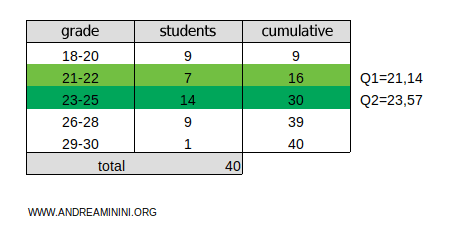
Note: Using the midpoint method, the second quartile would be Q₂=24, where 24 is the midpoint of the class 23-25.

To calculate the third quartile (Q₃), multiply the total cumulative frequency f_tot=40 by 3/4:

$$ k =f_{tot} \cdot \frac{3}{4} = 40 \cdot \frac{3}{4} = 30 $$

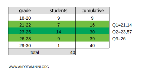
The result, 30, lies within the cumulative frequency range 30-39 for the class 26-28.

Once again, linear interpolation is used to find the exact value of the third quartile:

$$ Q_3 = x_{inf} + (x_{sup} - x_{inf}) \cdot \frac{c - n_{prec}}{n_{classe}} $$

Here’s what the terms mean:

• x_inf=26 and x_sup=28 are the boundaries of the class 26-28.
• c=30 is the position of the third quartile.
• n_classe=9 is the frequency of the class 26-28.
• n_prec=30 is the cumulative frequency of the classes preceding 26-28.

Substitute the values and calculate:

$$ Q_3 = 26 + (28 - 26) \cdot \frac{30 - 30}{9} $$

$$ Q_3 = 26 + 2 \cdot \frac{0}{9} $$

$$ Q_3 = 26 $$

Therefore, the third quartile is Q₃=26.

The interquartile range

The interquartile range is the difference between the third quartile (Q₃) and the first quartile (Q₁): $$ Q_3 - Q_1 $$

For example, if the quartiles of a data set are:

$$ Q_1 = 4.5 $$

$$ Q_2 = 6.5 $$

$$ Q_3 = 8.5 $$

The interquartile range is 4:

$$ Q_3 - Q_1 = 8.5 - 4.5 = 4 $$

And so on.