Bisection Method
The bisection method (also known as the zero-finding method) is a numerical technique used to find roots of a continuous function within an interval \([a, b]\), where the function changes sign.
In other words, it aims to find a point \( p \) such that \( f(p) = 0 \)-a root of the function \( f(x) \)-given that there's at least one root in the interval \([a, b]\).
$$ f(a) \cdot f(b) < 0 $$
Additionally, the function \( f \) must be continuous over the interval \([a, b] \).
How the method works
- Compute the midpoint \( p = \frac{a + b}{2} \)
- Evaluate \( f(p) \)
- Depending on the sign of \( f(p) \), replace either \( a \) or \( b \) to isolate the subinterval where the sign change-and therefore the root-occurs
- Repeat the process (iterate) until one of the following stopping criteria is met:
- Absolute error: \( |p_n - p_{n-1}| < \varepsilon \)
- Relative error: \( \frac{|p_n - p_{n-1}|}{|p_n|} < \varepsilon \)
- Function value close to zero: \( |f(p_n)| < \varepsilon \)
This method is straightforward to implement and highly reliable, since it always converges when \( f(a) \cdot f(b) < 0 \).
However, it converges slowly and often requires many iterations to achieve a high level of precision.
It also requires that \( f(a) \) and \( f(b) \) have opposite signs, and it may overlook more accurate approximations along the way.
Note. The bisection method is an excellent first step for locating roots-especially when a good initial guess is unavailable. That said, for faster convergence and greater efficiency, it’s often complemented or replaced by more sophisticated methods such as Newton-Raphson or the secant method.
A Practical Example
Let’s walk through a step-by-step example of the bisection method applied to a function.
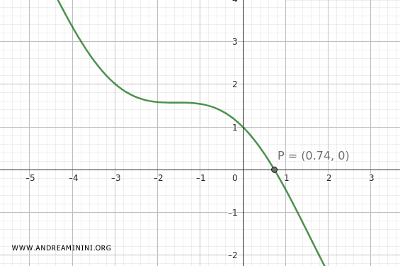
We want to find a root of the function \( f(x) = \cos(x) - x \) in the interval \([0, 1]\).
First, we check that the function has opposite signs at the endpoints of the interval:
$$ f(0) = \cos(0) - 0 = 1 $$
$$ f(1) = \cos(1) - 1 \approx 0.5403 - 1 = -0.4597 $$
Since \( f(0) \cdot f(1) < 0 \), there must be at least one root in the interval \([0, 1]\).
We set a tolerance of \( \text{TOL} = 0.001 \) to achieve three-decimal-place accuracy.
Here are the initial iterations:
| n | a | b | p = (a + b)/2 | f(p) = cos(x)-x | Chosen Interval |
|---|---|---|---|---|---|
| 1 | 0.000 | 1.000 | 0.500 | cos(0.5) - 0.5 ≈ 0.3776 | f(p) > 0 ⇒ [0.5, 1] |
| 2 | 0.500 | 1.000 | 0.750 | cos(0.75) - 0.75 ≈ -0.0183 | f(p) < 0 ⇒ [0.5, 0.75] |
| 3 | 0.500 | 0.750 | 0.625 | cos(0.625) - 0.625 ≈ 0.1850 | f(p) > 0 ⇒ [0.625, 0.75] |
| 4 | 0.625 | 0.750 | 0.6875 | cos(0.6875) - 0.6875 ≈ 0.0844 | [0.6875, 0.75] |
| 5 | 0.6875 | 0.750 | 0.71875 | cos(0.71875) - 0.71875 ≈ 0.0333 | [0.71875, 0.75] |
| 6 | 0.71875 | 0.750 | 0.734375 | cos(0.734375) - 0.734375 ≈ 0.0073 | [0.734375, 0.75] |
| 7 | 0.734375 | 0.750 | 0.7421875 | cos(0.7421875) - 0.7421875 ≈ -0.0055 | [0.734375, 0.7421875] |
| 8 | 0.734375 | 0.7421875 | 0.73828125 | cos(0.73828125) - 0.73828125 ≈ 0.0009 ✅ | Stop! |
Explanation. In the first iteration (\( n = 1 \)), the midpoint is \( p = 0.5 \), and \( f(0.5) = \cos(0.5) - 0.5 = 0.3776 \). Since the value is positive, the root must lie to the right of 0.5, so we update the interval to \( [0.5, 1] \). In the second iteration, the midpoint is \( p = 0.750 \), and the function evaluates to a negative value \( f(0.75) = -0.0183 \). This indicates the root lies to the left of 0.75, so the interval becomes \( [0.5, 0.75] \). We continue this iterative process until we find a point \( p \) such that \( f(p) \) is within our error tolerance of ±0.001.
After 8 iterations, we’ve zeroed in on a solution with the desired precision:
\[ p \approx 0.73828125 \quad \text{with } |f(p)| < 0.001 \]
Thus, the root of \( \cos(x) = x \) is approximately 0.738-accurate to three decimal places.
Does it always work? The bisection method is guaranteed to work only if the function changes sign over the interval and is continuous (i.e., no gaps or discontinuities). If \( f(a) \cdot f(b) > 0 \), the method won't find the root-even if one exists. Also, it’s relatively slow compared to other techniques. One more caveat: you must first identify an interval where a root is known to exist, which isn’t always obvious. It's a bit like looking for your lost keys in the living room-it’s easy only if you already suspect they’re somewhere between the couch and the window.
Exploring the Domain: How to Identify Root-Containing Intervals
Exploring the domain of a function means identifying intervals \([a, b]\) where \( f(a) \cdot f(b) < 0 \)-in other words, where the function changes sign, indicating the presence of at least one root.
This is a crucial preliminary step before applying the bisection method.
In practice, it involves evaluating the function at a sequence of points across its domain and looking for consecutive pairs \( a \) and \( b \) such that the function changes sign between them-that is, \( f(a) \cdot f(b) < 0 \).
By the Intermediate Value Theorem, at least one root must exist in any such interval \([a, b]\).
The choice of spacing between evaluation points-known as the exploration step size-is critical because:
- If the step is too large, you risk skipping over sign changes and missing roots
- If the step is too small, you'll capture all the roots, but the computational cost increases significantly
So the goal is to strike a balance between accuracy and efficiency-using a fine enough step to capture meaningful behavior in the function, but not so fine that the process becomes unnecessarily burdensome.
Only after identifying sign-change intervals can we proceed to apply the bisection method within each one.
Example
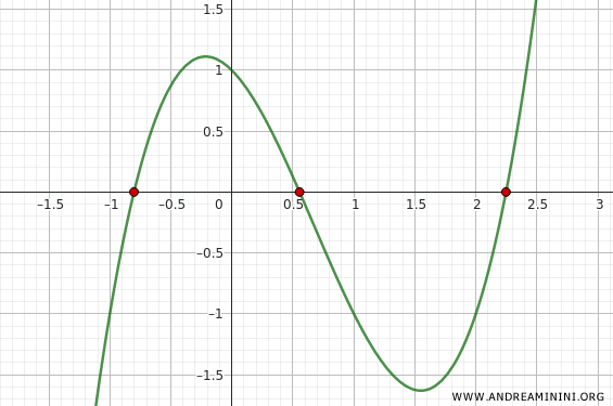
Let’s find all real roots of the function:
\[ f(x) = x^3 - 2x^2 - x + 1 \]
At the outset, we don’t know where the roots are. Since this is a third-degree polynomial, we know it can have up to three real roots-but we don’t know where they are, how many there actually are, or even if any of them are obvious.
There are no obvious integer roots, so we can’t rely on inspection. A numerical exploration is required.
Let’s start by evaluating the function at several points with an exploration step of 5:
\[
\begin{array}{c|c}
x & f(x) \\
\hline
-10 & -1189 \\
-5 & -169 \\
0 & 1 \\
5 & 71 \\
10 & 791 \\
\end{array}
\]
From the table, we can see there must be at least one root in the interval (-5, 0).
However, relying solely on this coarse analysis would be misleading-the step size is too large. We're “flying too high” over the function and could easily miss important changes in behavior.
So let’s reduce the step size to 1 to get a more detailed view.
\[
\begin{array}{cc}
x & f(x) \\
\hline
-5 & -169 \\
-4 & -91 \\
-3 & -41 \\
-2 & -13 \\
-1 & -1 \\
0 & 1 \\
1 & -1 \\
2 & -1 \\
3 & 7 \\
4 & 29 \\
5 & 71 \\
\end{array}
\]
Now we can clearly see three sign changes: one in the interval (-1, 0), another in (0, 1), and a third in (2, 3).
Note. This shows that using large step sizes might cause you to overlook roots that lie between the sampled points. On the other hand, using a very small step size guarantees that you’ll catch all roots-but at the cost of much more computation. For example, using a step of 0.1 over the interval \([-10, 10]\) would require 200 evaluations-far too many. As always, moderation is key. A well-chosen step, like 0.5 or 0.25, depending on the function, usually offers a good trade-off.
Once we've identified the sign-change intervals, we can apply the bisection method within each:
- First interval: \([-1, 0]\)
After just a few iterations, we approximate a root: \[ x_1 \approx -0.8 \] - Second interval: \([0, 1]\)
Again, only a handful of iterations are needed to reach: \[ x_2 \approx 0.5 \] - Third interval: \([2, 3]\)
Applying bisection here yields: \[ x_3 \approx 2.2 \]
So, the three approximate real roots of the function \( f(x) = x^3 - 2x^2 - x + 1 \) are \( x_1 \approx -0.8 \), \( x_2 \approx 0.5 \), and \( x_3 \approx 2.2 \).
In conclusion, domain exploration is a critical step when locating root intervals before applying the bisection method.
You need a balanced step size, not too large, not too small.
Once intervals with a sign change have been found, the bisection method can be applied locally-reliably and efficiently.
And so on.


