Numerical Computation

What is Numerical Computation?

Numerical computation is a branch of mathematics dedicated to solving problems through computational algorithms.

What is it used for?

Numerical computation helps us find approximate solutions to complex problems that are difficult or even impossible to tackle with traditional mathematical analysis.

The slight loss in precision is often outweighed by the speed of calculation.

This approach is especially useful in engineering and scientific fields.

Note: Numerical computation is frequently used to solve systems of linear equations, in linear programming to minimize a function with specific constraints, for optimizing functions of multiple variables, and in differential calculus (integrals, derivatives, differential equations).

Difference between Numerical Computation and Numerical Analysis

While sometimes used interchangeably, numerical computation and numerical analysis have distinct meanings.

• Numerical computation focuses on creating algorithms for solving problems in continuous mathematics (e.g., finding an approximate solution to a definite integral or a differential equation).
• Numerical analysis dives deeper into the mathematical study of these algorithms, evaluating their properties and behavior.

A Practical Example

Below are some real-world applications of numerical computation:

Example 1

Many differential equations are too complex to solve directly.

Numerical computation provides an approximate solution, which is useful when a small margin of error is acceptable.

Example 2

Numerical computation can also estimate the area of a shape without needing to calculate the exact integral.

Discretizing Continuous Problems

Numerical computation often involves discretizing a continuous problem, which means building a discrete model to represent a real-world phenomenon in a finite numerical space.

Many real-world situations can be represented by a mathematical model.

A mathematical model consists of variables, constraints, functional relationships, and parameters that define the problem.

A mathematical model is reliable if it is:

• well-posed
  yielding unique, stable solutions that vary smoothly with changes in input. For example, under consistent conditions, the model produces consistent results.
• well-conditioned
  meaning that small changes in input data lead to small changes in output. For instance, minor data rounding won’t significantly affect the model’s results.

However, mathematical models often approach the problem in continuous mathematics, which can make solution-finding computationally demanding.

To overcome this, we can rewrite the model in discrete form using non-continuous numerical values.

This discrete model (or numerical model) yields an approximate solution but usually requires less computational time.

Note: Existence, uniqueness, and stability conditions are met in the discrete model too. The discrete model remains well-posed and well-conditioned like the continuous model. However, it’s only useful if the approximate solution falls within an acceptable error margin.

Methods in Numerical Computation

There are two main approaches to numerical computation:

• Direct methods
  These use algorithms to reach a solution in a predetermined number of steps, like the Sieve of Eratosthenes.
• Iterative methods
  These involve successive approximations that converge on a final solution, such as estimating a function’s integral using the rectangle method.

The Sieve of Eratosthenes

The Sieve of Eratosthenes is an algorithm for finding all prime numbers between 1 and N.

How does it work?

The algorithm lists all natural numbers from 1 to N.

$$ 1 \ , \ 2 \ , \ 3 \ , \ 4 \ , \ 5 \ , \ 6 \ , \ 7 \ , \ 8 \ , \ 9 \ , \ ... \ , \ N $$

Then, it removes any numbers that aren’t prime.

Each number is checked individually and divided by all previous numbers.

• If the number is divisible by any number other than 1, it is removed from the list.

  Example: The algorithm checks number 6. Dividing it by 2 leaves no remainder, so it’s removed from the list. The next number (7) is then analyzed.

• If the number is divisible only by one, it remains on the list, and the algorithm moves to the next number.

  Example: The algorithm checks number 5. Dividing it by 2 leaves a remainder of 1, and division by 3 and 4 also results in remainders. Since 5 isn’t divisible by any other numbers except 1, it’s considered prime.

At the end of this process, only prime numbers from 1 to N remain in the list.

$$ 1 \ , \ 2 \ , \ 3 \ , \ 5 \ , \ 7 \ , \ ... \ , \ N $$

The Rectangle Method for Calculating a Definite Integral

The rectangle method approximates the definite integral of a function.

How does it work?

We consider the function over a defined interval (a,b).

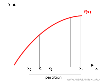
The interval (a,b) is then split into n smaller segments of equal length.

This creates a partition over the interval.

For each segment in this partition, the height is determined from one of the endpoints, as the perpendicular segment connecting the x-axis to the function’s graph.

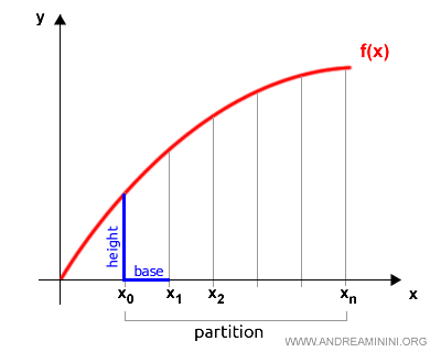
The length of the segment (base) is multiplied by the height to find each rectangle’s area.

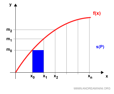
We then move on to the next segment.

The total area of all rectangles approximates the value of the definite integral over (a,b).

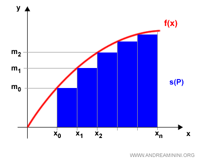
This approximation is a lower estimate since we calculated the height from the left endpoint of each interval.

Note: Using the right endpoint instead would yield an upper estimate of the definite integral.

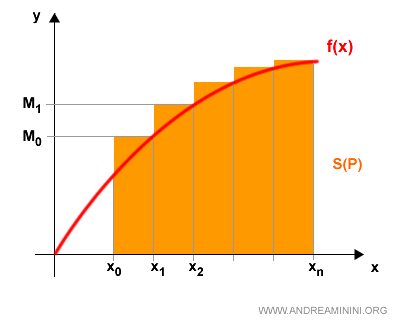
The accuracy of the approximation improves as the segments become smaller and more numerous.

And so forth.