Critical Values in the Normal Distribution

In a normal distribution, critical values refer to the \( z \) values that define the tails of the distribution.

These values are essential for determining confidence intervals and conducting hypothesis tests.

In a standardized normal distribution (where the mean is \( \mu = 0 \) and the standard deviation is \( \sigma = 1 \)), critical values correspond to the \( z \) scores at which the cumulative probability reaches a specific threshold.

Here are some of the most commonly used critical values for confidence intervals and statistical testing:

• 68.27% confidence: \( z = \pm 1 \)
• 90% confidence: \( z = \pm 1.645 \)
• 95% confidence: \( z = \pm 1.96 \)
• 95.45% confidence: \( z = \pm 2 \)
• 99% confidence: \( z = \pm 2.576 \)
• 99.74% confidence: \( z = \pm 3 \)
• 99.9% confidence: \( z = \pm 3.291 \)

For example, the critical value \( z = \pm 1.645 \) marks the range within which 90% of values fall around the mean in a standard normal distribution, leaving 5% in each tail.

Critical values help to establish how far from the mean a parameter is expected to fall, within a specified confidence level (e.g., 95%).

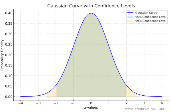
They’re also used to assess whether an observed result is statistically significant by comparing it to the relevant critical value.

The Normal Distribution Table

The integral of the normal distribution's density function (the area under the curve) cannot be solved using basic methods or simple formulas.

If you need to find a critical value for a different confidence level, you can refer to the critical values table:

z	0.00	0.01	0.02	0.03	0.04	0.05	0.06	0.07	0.08	0.09
-3.4	0.0003	0.0003	0.0003	0.0003	0.0003	0.0003	0.0003	0.0003	0.0003	0.0002
-3.3	0.0005	0.0005	0.0005	0.0004	0.0004	0.0004	0.0004	0.0004	0.0004	0.0003
-3.2	0.0007	0.0007	0.0006	0.0006	0.0006	0.0006	0.0006	0.0005	0.0005	0.0005
-3.1	0.0010	0.0009	0.0009	0.0009	0.0008	0.0008	0.0008	0.0008	0.0007	0.0007
-3.0	0.0013	0.0013	0.0013	0.0012	0.0012	0.0011	0.0011	0.0011	0.0010	0.0010
-2.9	0.0019	0.0018	0.0018	0.0017	0.0016	0.0016	0.0015	0.0015	0.0014	0.0014
-2.8	0.0026	0.0025	0.0024	0.0023	0.0023	0.0022	0.0021	0.0021	0.0020	0.0019
-2.7	0.0035	0.0034	0.0033	0.0032	0.0031	0.0030	0.0029	0.0028	0.0027	0.0026
-2.6	0.0047	0.0045	0.0044	0.0043	0.0041	0.0040	0.0039	0.0038	0.0037	0.0036
-2.5	0.0062	0.0060	0.0059	0.0057	0.0055	0.0054	0.0052	0.0051	0.0049	0.0048
-2.4	0.0082	0.0080	0.0078	0.0075	0.0073	0.0071	0.0069	0.0068	0.0066	0.0064
-2.3	0.0107	0.0104	0.0102	0.0099	0.0096	0.0094	0.0091	0.0089	0.0087	0.0084
-2.2	0.0139	0.0136	0.0132	0.0129	0.0125	0.0122	0.0119	0.0116	0.0113	0.0110
-2.1	0.0179	0.0174	0.0170	0.0166	0.0162	0.0158	0.0154	0.0150	0.0146	0.0143
-2.0	0.0228	0.0222	0.0217	0.0212	0.0207	0.0202	0.0197	0.0192	0.0188	0.0183
-1.9	0.0287	0.0281	0.0274	0.0268	0.0262	0.0256	0.0250	0.0244	0.0239	0.0233
-1.8	0.0359	0.0351	0.0344	0.0336	0.0329	0.0322	0.0314	0.0307	0.0301	0.0294
-1.7	0.0446	0.0436	0.0427	0.0418	0.0409	0.0401	0.0392	0.0384	0.0375	0.0367
-1.6	0.0548	0.0537	0.0526	0.0516	0.0505	0.0495	0.0485	0.0475	0.0465	0.0455
-1.5	0.0668	0.0655	0.0643	0.0630	0.0618	0.0606	0.0594	0.0582	0.0571	0.0559
-1.4	0.0808	0.0793	0.0778	0.0764	0.0749	0.0735	0.0721	0.0708	0.0694	0.0681
-1.3	0.0968	0.0951	0.0934	0.0918	0.0901	0.0885	0.0869	0.0853	0.0838	0.0823
-1.2	0.1151	0.1131	0.1112	0.1093	0.1075	0.1056	0.1038	0.1020	0.1003	0.0985
-1.1	0.1357	0.1335	0.1314	0.1292	0.1271	0.1251	0.1230	0.1210	0.1190	0.1170
-1.0	0.1587	0.1562	0.1539	0.1515	0.1492	0.1469	0.1446	0.1423	0.1401	0.1379
-0.9	0.1841	0.1814	0.1788	0.1762	0.1736	0.1711	0.1685	0.1660	0.1635	0.1611
-0.8	0.2119	0.2090	0.2061	0.2033	0.2005	0.1977	0.1949	0.1922	0.1894	0.1867
-0.7	0.2420	0.2389	0.2358	0.2327	0.2296	0.2266	0.2236	0.2206	0.2177	0.2148
-0.6	0.2743	0.2709	0.2676	0.2643	0.2611	0.2578	0.2546	0.2514	0.2483	0.2451
-0.5	0.3085	0.3050	0.3015	0.2981	0.2946	0.2912	0.2877	0.2843	0.2810	0.2776
-0.4	0.3446	0.3409	0.3372	0.3336	0.3300	0.3264	0.3228	0.3192	0.3156	0.3121
-0.3	0.3821	0.3783	0.3745	0.3707	0.3669	0.3632	0.3594	0.3557	0.3520	0.3483
-0.2	0.4207	0.4168	0.4129	0.4090	0.4052	0.4013	0.3974	0.3936	0.3897	0.3859
-0.1	0.4602	0.4562	0.4522	0.4483	0.4443	0.4404	0.4364	0.4325	0.4286	0.4247
0.0	0.5000	0.4960	0.4920	0.4880	0.4840	0.4801	0.4761	0.4721	0.4681	0.4641
0.1	0.5398	0.5438	0.5478	0.5517	0.5557	0.5596	0.5636	0.5675	0.5714	0.5753
0.2	0.5793	0.5832	0.5871	0.5910	0.5948	0.5987	0.6026	0.6064	0.6103	0.6141
0.3	0.6179	0.6217	0.6255	0.6293	0.6331	0.6368	0.6406	0.6443	0.6480	0.6517
0.4	0.6554	0.6591	0.6628	0.6664	0.6700	0.6736	0.6772	0.6808	0.6844	0.6879
0.5	0.6915	0.6950	0.6985	0.7019	0.7054	0.7088	0.7123	0.7157	0.7190	0.7224
0.6	0.7257	0.7291	0.7324	0.7357	0.7389	0.7422	0.7454	0.7486	0.7517	0.7549
0.7	0.7580	0.7611	0.7642	0.7673	0.7704	0.7734	0.7764	0.7794	0.7823	0.7852
0.8	0.7881	0.7910	0.7939	0.7967	0.7995	0.8023	0.8051	0.8078	0.8106	0.8133
0.9	0.8159	0.8186	0.8212	0.8238	0.8264	0.8289	0.8315	0.8340	0.8365	0.8389
1.0	0.8413	0.8438	0.8461	0.8485	0.8508	0.8531	0.8554	0.8577	0.8599	0.8621
1.1	0.8643	0.8665	0.8686	0.8708	0.8729	0.8749	0.8770	0.8790	0.8810	0.8830
1.2	0.8849	0.8869	0.8888	0.8907	0.8925	0.8944	0.8962	0.8980	0.8997	0.9015
1.3	0.9032	0.9049	0.9066	0.9082	0.9099	0.9115	0.9131	0.9147	0.9162	0.9177
1.4	0.9192	0.9207	0.9222	0.9236	0.9251	0.9265	0.9279	0.9292	0.9306	0.9319
1.5	0.9332	0.9345	0.9357	0.9370	0.9382	0.9394	0.9406	0.9418	0.9429	0.9441
1.6	0.9452	0.9463	0.9474	0.9484	0.9495	0.9505	0.9515	0.9525	0.9535	0.9545
1.7	0.9554	0.9564	0.9573	0.9582	0.9591	0.9599	0.9608	0.9616	0.9625	0.9633
1.8	0.9641	0.9649	0.9656	0.9664	0.9671	0.9678	0.9686	0.9693	0.9699	0.9706
1.9	0.9713	0.9719	0.9726	0.9732	0.9738	0.9744	0.9750	0.9756	0.9761	0.9767
2.0	0.9772	0.9778	0.9783	0.9788	0.9793	0.9798	0.9803	0.9808	0.9812	0.9817
2.1	0.9821	0.9826	0.9830	0.9834	0.9838	0.9842	0.9846	0.9850	0.9854	0.9857
2.2	0.9861	0.9864	0.9868	0.9871	0.9875	0.9878	0.9881	0.9884	0.9887	0.9890
2.3	0.9893	0.9896	0.9898	0.9901	0.9904	0.9906	0.9909	0.9911	0.9913	0.9916
2.4	0.9918	0.9920	0.9922	0.9925	0.9927	0.9929	0.9931	0.9932	0.9934	0.9936
2.5	0.9938	0.9940	0.9941	0.9943	0.9945	0.9946	0.9948	0.9949	0.9951	0.9952
2.6	0.9953	0.9955	0.9956	0.9957	0.9959	0.9960	0.9961	0.9962	0.9963	0.9964
2.7	0.9965	0.9966	0.9967	0.9968	0.9969	0.9970	0.9971	0.9972	0.9973	0.9974
2.8	0.9974	0.9975	0.9976	0.9977	0.9977	0.9978	0.9979	0.9979	0.9980	0.9981
2.9	0.9981	0.9982	0.9982	0.9983	0.9984	0.9984	0.9985	0.9985	0.9986	0.9986
3.0	0.9987	0.9987	0.9987	0.9988	0.9988	0.9989	0.9989	0.9989	0.9990	0.9990
3.1	0.9990	0.9991	0.9991	0.9991	0.9992	0.9992	0.9992	0.9992	0.9993	0.9993
3.2	0.9993	0.9993	0.9994	0.9994	0.9994	0.9994	0.9994	0.9995	0.9995	0.9995
3.3	0.9995	0.9995	0.9995	0.9996	0.9996	0.9996	0.9996	0.9996	0.9996	0.9997
3.4	0.9997	0.9997	0.9997	0.9997	0.9997	0.9997	0.9997	0.9997	0.9997	0.9998

This table provides critical values for the area under the Gaussian curve starting from -∞.

Graphically, with the total area under the curve set to 1, the \( z \) value identifies the area under the curve starting from the left.

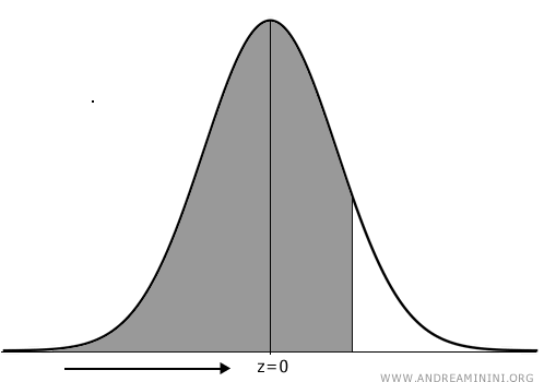
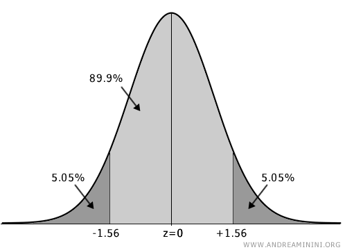
For instance, take the cell with the value "0.0505," which represents 5.05% of the area under the curve from the left.

This cell corresponds to row \( X = -1.6 \) and column \( Y = 0.4 \).

The critical value is calculated by adding these row and column values, resulting in:

$$ z = X + Y = -1.6 + 0.4 = -1.56 $$

Thus, the critical values are \( z = -1.56 \) and its opposite, \( z = 1.56 \).

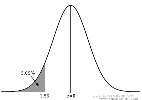
Since the area under the left tail of the curve (5.05%) matches that of the right tail (5.05%), the total area for both tails is 10.1%, 

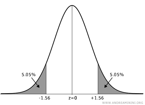
indicating that the critical value \( z = \pm 1.56 \) defines a confidence interval around the mean (z = 0) of 100% - 10.1% = 89.9%.

This approach enables you to find the critical value for any confidence interval.

Example Calculation

Let’s calculate the critical value for a 95% confidence level.

This means there’s a complementary probability of 5%, split equally between the two tails, so each tail has 2.5%.

The total area in both tails is:

$$ 1 - 0.95 = 0.05 $$

Dividing the area for each tail:

$$ 0.05 / 2 = 0.025 $$

Now, I need to find a \( z \) value that leaves 1 - 0.025 = 0.975 of the area to its left (97.5% of the distribution falls to the left of \( z \)).

Once the tail probability is identified, I look for a critical value \( z \) such that \( P(Z \leq z) = 0.975 \).

$$ z = X + Y $$

The value of 0.975 corresponds to row \( X = 1.9 \) and column \( Y = 0.6 \), matching exactly what we’re looking for.

Therefore, the critical value is \( z \approx 1.96 \).

$$ z = X + Y = 1.9 + 0.6 = 1.96 $$

In summary, for a 95% confidence level, the appropriate critical value is \( z = 1.96 \).

Methods for Finding Critical Values

There are several ways to find critical values:

• Normal Distribution Tables: These tables show critical \( z \) values for various probability levels.
• Scientific Calculators: Many calculators allow for direct computation of normal distribution quantiles.
• Statistical Software: Tools like Excel, R, Python, and other statistical software offer functions to calculate normal distribution quantiles. For example, in Python, you can use the norm.ppf() function from the scipy.stats library to find \( z \) for a given cumulative probability.

And so forth.