Normal Distribution
What is the normal distribution?
The normal distribution is a probability distribution defined by a symmetrical bell-shaped curve. It’s also known as the Gaussian distribution.
This bell-shaped curve is referred to as the normal curve or Gaussian curve.
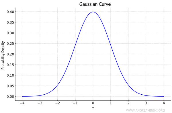
The normal distribution is determined by the mean and standard deviation of a population.
Note: The term "Gaussian" comes from the German mathematician Carl Friedrich Gauss, who first described it in 1809. In mathematics and statistics, the term "normal distribution" is more commonly used, while "Gaussian distribution" is favored in physics and engineering. Both refer to the same continuous probability distribution.
How is it calculated?
To calculate the normal distribution of a population, you need two key pieces of data:
With these two values, you can calculate the probability of different outcomes.
What is it used for?
The normal distribution allows us to understand the likelihood of different values a statistical variable can take.
Example: The height of individuals within a certain age group is often well represented by a normal distribution, as most people tend to have heights close to the average. However, not all phenomena follow a Gaussian distribution, and there is always some degree of uncertainty in the representation.
Characteristics of the Gaussian Distribution
In a Gaussian distribution, 68.27% of values lie between M-σ and M+σ, where M is the mean and σ is the standard deviation.
This occurs because, in a Gaussian distribution, the standard deviation is closely related to how values are distributed around the mean.
It can be shown that:
- 68.27% of values are between M-σ and M+σ, which corresponds to one standard deviation from the mean
- 95.45% of values are between M-2σ and M+2σ, or within two standard deviations of the mean
- 99.74% of values are between M-3σ and M+3σ, or within three standard deviations of the mean
To encompass 99.99% of values, you need to consider the range between M-3.29σ and M+3.29σ.
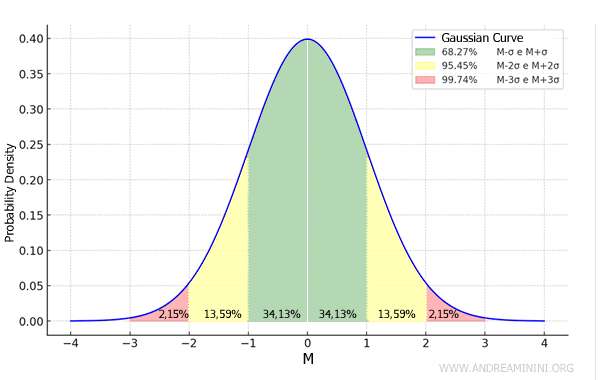
This is known as the empirical rule, or the "68-95-99.7 rule" of the Gaussian distribution.
Note: The results obtained by applying this rule to a dataset are approximations, as real populations don’t perfectly follow the normal distribution. However, for many phenomena, the results are reasonably accurate.
Critical (z) Values of the Normal Distribution
Each confidence level (or cumulative probability) is associated with a critical value (z), which represents the number of standard deviations away from the mean required to encompass a certain percentage of the area under the curve.
For instance, if 68.27% of the values lie between M-σ and M+σ, the critical value is z=1. This indicates that approximately 68.27% of the values in a standard normal distribution fall within 1 standard deviation of the mean $ M \pm \sigma $. If 95.45% of the values are between M-2σ and M+2σ, the critical value is z=2. Similarly, if 99.74% of the values fall between M-3σ and M+3σ, the critical value is z=3. And so forth.
These critical values are essential for constructing confidence intervals and have various other applications in statistics, particularly when the data follow a normal distribution.
Below are some of the most commonly used critical values:
- 90% confidence level: z=1.645
- 95% confidence level: z=1.96
- 99% confidence level: z=2.575
- 99.9% confidence level: z=3.291
To find the critical (z) value for a different confidence level, you can refer to the standard normal distribution table.
The Probability Density Function
The general formula for the probability density function of a normal distribution (Gaussian curve) is:
$$ f(x) = \frac{1}{\sigma \sqrt{2\pi}} \, e^{-\frac{(x - M)^2}{2 \sigma ^2}} $$
where:
- \( M \) is the mean of the distribution,
- \(\sigma \) is the standard deviation,
- \( x \) is the random variable,
- \( e \) is the base of the natural logarithm (\( \approx 2.718 \)).
This formula describes how the values of \( x \) are distributed around the mean \( M \), with the spread determined by the standard deviation \(\sigma\).

Comparing Two Distributions with the Same Mean but Different Standard Deviations
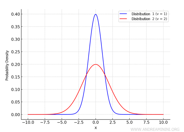
When two distributions share the same mean \( M \) but have different standard deviations \( \sigma \), the one with the larger standard deviation will be broader and flatter along the horizontal axis.
This is because the standard deviation measures how spread out the data is around the mean: a larger value means the data is more dispersed, resulting in a wider, lower curve.
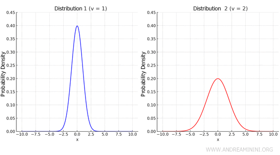
On the other hand, a smaller standard deviation means the data is more concentrated around the mean, making the curve narrower and taller.
Both curves, however, cover the same total area beneath them, equal to 1, as they represent probability distributions.
This visual difference reflects how the standard deviation influences data variability in the distribution.
Example: Let’s compare two normal distributions, both with a mean of \( M = 0 \), but with different standard deviations:
- Distribution 1: \( M = 0 \) and \( \sigma = 1 \)
- Distribution 2: \( M = 0 \) and \( \sigma = 2 \)
We can analyze how these distributions appear graphically and how their shape changes based on their standard deviations.
- Distribution 1: \( N(0, 1) \)
This distribution has a standard deviation of 1. Its probability density function is:
\[ f_1(x) = \frac{1}{\sqrt{2\pi}} e^{-\frac{x^2}{2}} \]
This distribution is centered at \( M = 0 \), and the data is more concentrated around the mean. The curve will be narrower and taller. - Distribution 2: \( N(0, 2) \)
This distribution has a standard deviation of 2. Its probability density function is:
\[ f_2(x) = \frac{1}{2\sqrt{2\pi}} e^{-\frac{x^2}{8}} \]
This distribution is also centered at \( M = 0 \), but since the standard deviation is larger, the data is more spread out. The curve will be wider and flatter.
Thus, Distribution 1 (with \( \sigma = 1 \)) will have a narrower, taller curve, with data concentrated near the mean. Distribution 2 (with \( \sigma = 2 \)) will have a wider, flatter curve, with data spread out over a larger range.
A Practical Example
Consider a population X of 100 students, where the average height is known:
$$ \mu = 1.8 \ meters $$
and the standard deviation is:
$$ \sigma^2 = 0.1 $$
We want to use this information to calculate the probability of different height ranges.
Here’s a table showing heights in ascending order from 1.65 to 2.00 meters:
| Height | Probability Density | Cumulative |
|---|---|---|
| 1.60 | ||
| 1.65 | ||
| 1.70 | ||
| 1.75 | ||
| 1.80 | ||
| 1.85 | ||
| 1.90 | ||
| 1.95 | ||
| 2.00 |
Next, we calculate the normal and cumulative probability densities using the normal distribution.
| Height | Probability Density | Cumulative |
|---|---|---|
| 1.60 | 0.54 | 0.02 |
| 1.65 | 1.30 | 0.07 |
| 1.70 | 2.42 | 0.16 |
| 1.75 | 3.52 | 0.31 |
| 1.80 | 3.99 | 0.50 |
| 1.85 | 3.52 | 0.69 |
| 1.90 | 2.42 | 0.84 |
| 1.95 | 1.30 | 0.93 |
| 2.00 | 0.54 | 0.98 |
The probability density function provides an estimate of how likely different values are to occur.
For example, values closer to the mean (μ = 1.8) have a higher probability density.
Graphically, the probability density function forms the familiar shape of a symmetrical bell curve.
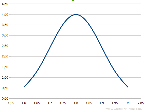
The cumulative distribution function, on the other hand, is an upward-sloping curve that rises from 0 to 1, where 0 and 1 represent probabilities.
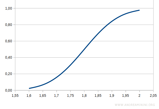
The cumulative distribution function helps us calculate the probability for specific ranges of heights.
For instance, if we know that the cumulative probability up to 1.7 meters is 0.16 and the probability up to 1.75 meters is 0.31, we can find the probability for the 1.7-1.75 meter range by taking the difference:
$$ p = 0.31 - 0.16 = 0.15 $$
Thus, the probability of having a height between 1.7 and 1.75 meters is 15%.
We can calculate the probabilities for other height ranges in a similar way.
| Height Range | Probability | Note |
|---|---|---|
| 1.60 - 1.65 | 0.05 | 0.07 - 0.02 = 0.05 = 5% |
| 1.65 - 1.70 | 0.09 | 0.16 - 0.07 = 0.09 = 9% |
| 1.70 - 1.75 | 0.15 | 0.31 - 0.16 = 0.15 = 15% |
| 1.75 - 1.80 | 0.19 | 0.50 - 0.31 = 0.19 = 19% |
| 1.80 - 1.85 | 0.19 | 0.69 - 0.50 = 0.19 = 19% |
| 1.85 - 1.90 | 0.15 | 0.84 - 0.69 = 0.15 = 15% |
| 1.90 - 1.95 | 0.09 | 0.93 - 0.84 = 0.09 = 9% |
| 1.95 - 2.00 | 0.05 | 0.98 - 0.93 = 0.05 = 5% |
Sample Analysis
The normal distribution allows us to study the characteristics of a population by analyzing just a sample of it.
What is a sample? A sample is a subset of data selected randomly from a population. The goal of sampling is to draw conclusions about the larger population based on the data collected from the sample, which helps save time and reduce the cost of statistical analysis.
In this case, the sample size is smaller than the total population size.
To conduct a sample analysis, we use:
- The sample mean (μc)
- The sample standard deviation (sc)
Note: For samples, we use the symbol "s" to represent the sample standard deviation, to distinguish it from the symbol σ, which is used to denote the standard deviation of a population.
The sample mean provides an approximation of the population mean.
This allows us to gain insight into the population without analyzing every individual in the dataset.
Note: Each sample has a slightly different mean, so sample analysis is subject to a margin of uncertainty that must be considered.
To quantify this uncertainty, we calculate the standard error.
$$ s_x = \frac{s_c}{ \sqrt{n-1} } $$
Where n is the sample size and sc is the sample standard deviation.
The standard error allows us to calculate the confidence interval.
$$ ( μ_c - 3 \cdot s_x \ , \ μ_c + 3 \cdot s_x ) $$
The confidence interval represents a range where, with 99.74% certainty, the true population mean is expected to fall.
Example: In a factory producing bolts, I take a sample of 50 bolts and measure their weight in grams. The sample mean is 19.3 grams, and the sample standard deviation is 0.985. In this case, the standard error is 0.14:
$$ s_x = \frac{0,985}{\sqrt{50-1}{}} = 0,14 $$
Therefore, the confidence interval is:
$$ (19,3 - 3 \cdot 0,14 \ , \ 19,3 + 3 \cdot 0,14 ) $$
$$ (18,88 \ , \ 19,72 ) $$
This means that with 99.75% confidence, the mean weight of the bolts in the entire population is between 18.88 grams and 19.72 grams.
If the estimate involves a percentage, a different formula is used to calculate the standard error:
$$ s = \sqrt{ \frac{f \cdot (1-f) }{n} } $$
In this case, too, the standard error is inversely related to the sample size (n).
As the sample size increases, the standard error decreases, and the confidence interval becomes narrower.
Example: In a jar containing a thousand balls, I take a sample of 50 and observe their color. 30% of the balls are red. To project this percentage to the entire population, I use the formula:
$$ s = \sqrt{ \frac{f \cdot (1-f) }{n} } $$
In this case, f=0.30 and n=50:
$$ s = \sqrt{ \frac{0.30 \cdot (1-0.30) }{50} } = \sqrt{ \frac{0.30 \cdot 0.70 }{50} } = \sqrt{ 0.21 }{50} = \sqrt{ 0.0042 } = 0.064 $$
The standard error is 0.064 percentage points. Therefore, the confidence interval is:
$$ (0.30 - 3 \cdot 0.064 \ , \ 0.30 + 3 \cdot 0.064 ) $$
$$ (0.30 - 0.192 \ , \ 0.30 - 0.192 ) $$
$$ (0.10,8 \ , \ 0.494 ) $$
This means that, with 99.74% confidence, the percentage of red balls in the entire population is between 10.8% and 49.4%. To reduce the range, I would need to take a larger sample. For example, if I take a sample of 200 balls, and 25% of them are red (f=0.25), I can calculate the standard error:
$$ s = \sqrt{ \frac{0.25 \cdot (1-0.25) }{200} } = 0.0306 $$
In this case, the confidence interval for the proportion of red balls in the population is between 15.9% and 34.1%:
$$ (0.25 - 0.0306 \cdot 3 \ , \ 0.25 + 0.0306 \cdot 3 ) $$
$$ (0.25 - 0.091 \ , \ 0.25 + 0.091 ) $$
$$ (0.159 \ , \ 0.341 ) $$
The range is still wide but narrower than in the previous example.
And so on.
