Sampling Distribution

The sampling distribution is the probability distribution of a statistic, such as the mean or variance, derived from multiple random samples of the same size taken from a population.

In other words, it shows how a particular statistic varies with different samples.

To create a sampling distribution, I follow these steps:

• Sampling
  I randomly select a certain number of samples from the population (N). Each sample must be the same size (n), meaning the same number of elements. For each sample, I calculate a statistic such as the sample mean, variance, etc. I repeat this process multiple times.
• Distribution of the statistic
  The statistics calculated for each sample will spread across a range of values. This is the sampling distribution of the statistic.

A common example is the sampling distribution of the mean: if I take many samples of a given size from a population and calculate the mean $ \bar{x} $ for each sample, I will get a distribution of sample means $ \bar{X} $ that typically approaches a normal or Gaussian distribution.

• The mean of the sampling distribution $ \mu_{ \bar{X} } $, or the average of all the sample means, is an estimate of the population mean $ \mu $.
• The standard error measures how much the values in the distribution deviate from the average $ \mu_{ \bar{X} } $. It’s calculated as  $$ \sigma_{ \bar{X} } = \frac{\sigma}{\sqrt{n}}  $$ where \( \sigma \) is the population standard deviation, and \( n \) is the sample size.

Sampling distributions are incredibly useful in inferential statistics because they allow me to estimate population parameters and calculate confidence intervals or run hypothesis tests.

Note. According to the central limit theorem, if the sample size is large enough, the sampling distribution of the sample mean will approach a normal distribution, regardless of the population's original distribution.

A practical example

Let’s say I need to determine the average height of all the students in a school, but I don’t have access to data for every student.

So, I decide to randomly sample groups of students and calculate the average height for each group.

Suppose the school has 1,000 students, and the population’s average height is 170 cm, with a standard deviation of 10 cm.

I randomly select samples of 30 students (with a sample size of \(n = 30\)) and calculate the average height for each sample.

Every time I take a new sample, I get a slightly different sample mean. For example:

• First sample: sample mean = 168 cm
• Second sample: sample mean = 172 cm
• Third sample: sample mean = 169 cm
• And so on...

After drawing several samples, I compile a list of all the sample means obtained.

These sample means form a new distribution, known as the sampling distribution of the mean.

Here’s a graph of the sampling distribution of the mean:

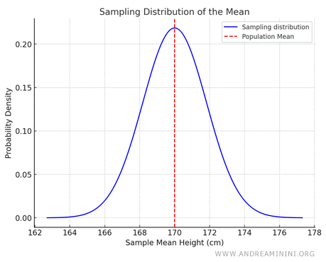
Note. The curve of the sampling distribution resembles a normal (Gaussian) distribution, where the dashed line represents the population mean (170 cm). The vertical axis shows how often a particular sample mean occurs.

The sampling distribution of means has these key characteristics:

• The mean of the sampling distribution is close to the population mean, i.e., 170 cm.
• The variance of the sampling distribution is smaller than the population variance. The standard deviation of the sampling distribution, called the standard error, is: $$ \sigma_{ \bar{X} } = \frac{\sigma}{ \sqrt{n}} $$ For example, if \( \sigma=10 \ cm \) and \( n=30 \)  the standard error is: $$ \sigma_{ \bar{X} } = \frac{10}{\sqrt{30}} \approx 1.83 \  cm $$ 

So even if the population’s height distribution isn't normal, thanks to the central limit theorem, the distribution of sample means will approximate a normal distribution.

The unbiased property of the sample mean

If I take all possible samples of a given size \(n\) from the population (or a very large number of random samples) and calculate the mean for each sample, the mean of all the sample means will be equal to the true population mean.

In other words, the average of all the sample means is the same as the population mean.

This is one of the fundamental principles of statistics and is based on the unbiasedness property of the sample mean.

Mathematically, if \( \mu \) is the population mean and \( \bar{x}_i \) is the mean of sample \(i\), then:

$$ \mathbb{E}(\bar{X}) = \mu $$

Where \( \mathbb{E}(\bar{X}) \) is the expected value of the sample mean, which equals the population mean \( \mu \).

This holds true for any sample size \(n\) and doesn’t depend on the population distribution, as long as the samples are independent and random.

This result shows that the sampling distribution is an unbiased estimator of the population mean.

What is an unbiased estimator? An unbiased estimator is a tool that, on average, gives me the true value of the parameter I’m trying to estimate. This means it doesn't introduce systematic errors, and as the number of samples increases, its results get closer to the true value.

In practice, it’s not necessary to collect all possible combinations of samples of a given size; it’s enough to take a large number of them.

The law of large numbers guarantees that even with just some of the samples, the average of the sample means will be very close to the population mean.

Example. If the sample size is \(n = 30\) and the population consists of \(N = 1000\) individuals, the sample space, in the case of sampling with replacement and ordered elements, consists of \(1000^{30}\) combinations. However, it’s not necessary to consider all possible combinations. With a sufficiently large number of random samples, I can achieve the same result, since the sample mean is an unbiased estimator of the population mean.

The central limit theorem

For random samples of sufficiently large size \(n\), the distribution of the sum or the sample mean \( \bar{X} \) tends to follow a normal distribution, regardless of the population’s original distribution, as long as the population’s variance \( \sigma^2 \) is finite.

In other words, as the sample size \(n\) increases, the distribution of the sample mean approaches a normal distribution, no matter the shape of the population distribution being sampled.

This happens because as the number of observations \( n \) increases, random variations tend to "cancel out," making the distribution of the sample mean more symmetric and bell-shaped (normal).

So even if the original population doesn’t follow a normal distribution, the mean of random samples will tend to.

Note. This property is extremely useful in statistics because it allows us to use the normal distribution for inference (like calculating confidence intervals and hypothesis testing) even when the population distribution is unknown.

And so on.