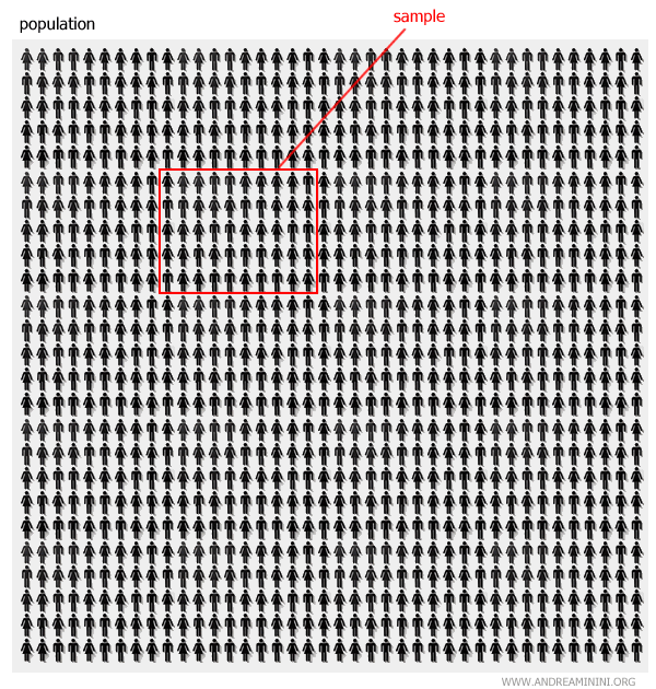
Sample in statistics

A sample is a subset of $n$ elements drawn from a larger population, referred to as the universe, with the aim of studying its key characteristics and inferring information about the entire population without needing to examine every individual.

It's essential that the sample be representative, meaning it accurately mirrors the characteristics of the universe it’s drawn from. In this case, it's known as a "stratified sample."

Only then can the conclusions from the sample be confidently generalized to the entire population.

Purpose of statistical sampling

A sample is used to estimate key parameters of the population, such as the mean, variance, or standard deviation.

Example: Suppose we want to estimate the average height of a population of trees in a forest. Instead of measuring every tree (the population), we could measure a sample of one hundred trees. If the sample is representative, the average height of the sample will be close to the average height of the entire forest, allowing us to make reliable conclusions about the population without measuring each tree. 

However, it's important to remember that sample estimates can differ from population values due to natural variability in the sample.

Generally, the larger the sample size (n), the more accurate the estimates are likely to be.

Sample size

Each sample consists of a certain number of elements, denoted by $n$.

The ratio of the sample size (n) to the population size (N) is called the "sampling rate."

$$ \frac{n}{N} $$

When the sample size is $n \leq 30$, it is considered a "small sample."

Sampling methods

Samples are selected from the population, and there are two main methods to do this:

• Sampling with replacement
  In this method, after an element is selected for the sample, it is returned to the population, allowing it to be selected again. This keeps the selection probability for each element constant.

  Example: If I randomly draw a card from a deck of 40 cards and then return it before drawing again, the probability of drawing any card remains the same for each draw, i.e., $P = \frac{1}{40}$.

• Sampling without replacement
  In this method, each element can only be selected once. After an element is drawn, it is removed from the pool, which changes the probabilities for the remaining elements.

  Example: If I draw a card from a deck of 40 cards without putting it back, the probability of drawing any specific card changes after each draw, as there are fewer cards left. For example, in the first draw the probability is $P = \frac{1}{40}$, but in the second draw it becomes $P = \frac{1}{39}$, and so on.

A practical example

Let’s say we want to estimate the average weight of students in a school with $N = 1000$ students.

We can’t practically weigh every student (the entire population), so we decide to take a sample of $n = 50$ students and use it to estimate the average weight of all the students in the school.

Let’s assume the weights (in kg) of the 50 students in the sample are as follows:

$$ 55,58,57,60,57,59,61,57,62,63,58,60,57,57,57,59,62,64,61,60,57,57,60,63,65,64,58,61,57,59,60,58,62,57,63,64,65,61,60,59,58,62,63,65,64,57,57,59,60,61 $$

The sample mean (denoted by \(\bar{x}\)) is calculated by summing all the weights and dividing by the number of students in the sample:

$$ \bar{x} = \frac{55 + 58 + 57 + 60 + \ldots + 61}{50} $$

$$ \bar{x} = \frac{3000}{50} = 60 \, \text{kg} $$

Thus, the sample mean is 60 kg.

Note: The sample mean is the average of the values in the sample. It is typically represented by $ \bar{x} $, while the population mean is denoted by $ \mu $.

Based on this sample, we can estimate that the average weight of all 1000 students is approximately 60 kg.

To measure the spread of the data, we can calculate the sample standard deviation (\(s\)) using the following formula, which gives the sum of squared deviations divided by \(n-1\):

$$ s = \sqrt{\frac{\sum_{i=1}^{n} (x_i - \bar{x})^2}{n-1}} $$

Where:

- \(x_i\) is the value of each individual weight,
- \(\bar{x}\) is the sample mean (60 kg in this case),
- \(n\) is the number of elements in the sample (50 in this case).

For simplicity, let’s assume the standard deviation calculation gives us \(s = 3.5\) kg.

This means that, on average, student weights deviate by about 3.5 kg from the mean.

If the sample was well-chosen, this provides a good estimate of both the average and variability for the entire population of 1000 students.

And so on.