Standard Deviation
Standard deviation (or root mean square deviation) is the square root of the arithmetic mean of the squared differences between each number and the mean. $$ \sigma = \sqrt{ \frac{1}{n} \cdot \sum_{i=1}^n (x_i- \mu)^2 } $$ Where μ is the mean, xi represents each element of the distribution, and n is the total number of elements. It is typically represented by the Greek letter sigma.
In other words, the standard deviation is the square root of the variance.
For frequency distributions, the formula to calculate the standard deviation is:
$$ \sigma = \sqrt{ \frac{1}{ \sum_{i=1}^k n_i} \cdot \sum_{i=1}^k (x_i- \mu)^2 \cdot n_i } $$
Where ni represents the frequency of each value, and the squared differences (xi - μ)2 from the mean are called squared deviations.
What is it used for?
The standard deviation (Std) is a measure of how much the data points spread out from the mean.
It is much more sensitive to small variations around the mean compared to the mean absolute deviation.
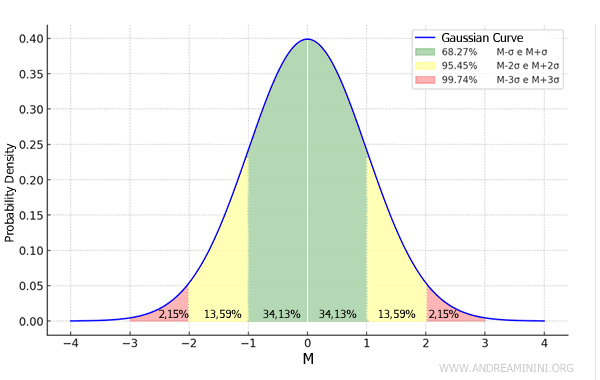
Note: Generally, about two-thirds of the elements in a distribution fall within the range (m - σ, m + σ). Almost all elements fall within the range (μ - 3σ, μ + 3σ).
A Practical Example
Example 1
This distribution consists of n=6 elements:
$$ 1 \ , \ 5 \ , \ 7 \ , \ 3 \ , \ 6 \ , \ 8 $$
The arithmetic mean of the distribution is μ = 5.
$$ \mu = \frac{1+5+7+3+6+8}{6 } = \frac{30}{6 } = 5 $$
Now, let’s calculate the variance of the distribution, knowing that n = 6 and μ = 5.
$$ \sigma^2 = \frac{1}{n} \cdot \sum_{i=1}^n (x_i - \mu )^2 $$
$$ \sigma^2 = \frac{1}{6} \cdot \sum_{i=1}^n (x_i - 5 )^2 $$
Breaking down the values: x1=1, x2=5, x3=7, x4=3, x5=6, x6=8
$$ \sigma^2 = \frac{1}{6} \cdot [ (1- 5 )^2+(5- 5 )^2+(7- 5 )^2+(3- 5 )^2+(6- 5 )^2+(8- 5 )^2] $$
$$ \sigma^2 = \frac{1}{6} \cdot [ (-4 )^2+(0 )^2+(2)^2+(-2)^2+(1)^2+(3)^2] $$
$$ \sigma^2 = \frac{1}{6} \cdot [ 16+0+4+4+1+9] $$
$$ \sigma^2 = \frac{34}{6} $$
The variance of the distribution is σ2 = 5.66.
$$ \sigma^2 = 5.66 $$
Thus, the standard deviation is the square root of 5.66.
$$ \sigma = \sqrt{5.66} = 2.34 $$
The standard deviation is 2.34.
Example 2
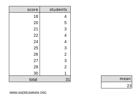
Here’s a frequency distribution:

We’ll calculate the weighted arithmetic mean of the distribution, which is μ = 23.
Now, let’s calculate the variance.
$$ \sigma^2 = \frac{1}{\sum_i^k n_i} \cdot \sum_{i=1}^k (x_i - \mu )^2 \cdot n_i $$
$$ \sigma^2 = \frac{1}{\sum_i^k n_i} \cdot \sum_{i=1}^k (x_i - 23 )^2 \cdot n_i $$
This distribution is divided into k=10 classes.
$$ \sigma^2 = \frac{1}{\sum_i^{10} n_i} \cdot \sum_{i=1}^{10} (x_i - 23 )^2 \cdot n_i $$
The sum of the frequencies Σni = 31.
$$ \sigma^2 = \frac{1}{31} \cdot \sum_{i=1}^{10} (x_i - 23 )^2 \cdot n_i $$
Now let’s calculate the squared deviations for each value x1 = 18, x2 = 20, x3 = 21, x4 = 22, x5 = 24, x6 = 25, x7 = 26, x8 = 27, x9 = 28, x10 = 30 from the mean μ = 23.
$$ \sigma^2 = \frac{(18 - 23 )^2 \cdot 4 + (20 - 23 )^2 \cdot 5 + (21 - 23 )^2 \cdot 3 + (22 - 23 )^2 \cdot 4 + (24 - 23 )^2 \cdot 4 + \\ + (25 - 23 )^2 \cdot 3 + (26 - 23 )^2 \cdot 2 + (27 - 23 )^2 \cdot 3 + (28 - 23 )^2 \cdot 2 + (30- 23 )^2 \cdot 1 }{31} $$
$$ \sigma^2 = \frac{(-5)^2 \cdot 4 + (-3)^2 \cdot 5 + (-2)^2 \cdot 3 + (-1)^2 \cdot 4 + (1)^2 \cdot 4 + \\ + (2)^2 \cdot 3 + (3)^2 \cdot 2 + (4)^2 \cdot 3 + (5)^2 \cdot 2 + (7)^2 \cdot 1 }{31} $$
$$ \sigma^2 = \frac{25 \cdot 4 +9 \cdot 5 + 4 \cdot 3 +1 \cdot 4 + 1 \cdot 4 +4 \cdot 3 + 9 \cdot 2 + 16 \cdot 3 + 25 \cdot 2 + 49 \cdot 1 }{31} $$
$$ \sigma^2 = \frac{100 + 45 + 12 + 4 + 4 + 12 + 18 + 48 + 50 + 49 }{31} $$
$$ \sigma^2 = \frac{342}{31} $$
The variance of the frequency distribution is σ2 = 11.03.
$$ \sigma^2 = 11.03 $$
Thus, the standard deviation is the square root of 11.03.
$$ \sigma = \sqrt{11.03} = 3.32 $$
What is the role of standard deviation?
Standard deviation measures how much the values in a data set deviate from the mean.
By comparing the standard deviations of two or more data sets, it helps me determine which one has greater variability.
Example. Suppose we have two classes of students who received grades on a scale from 1 to 10. In class A, the grades are 4, 5, 6, 6, 7, and 8, while in class B, the grades are 3, 3, 3, 9, 9, and 9. In both cases, the average grade is 6. $$ \mu_A = \frac{4+5+6+6+7+8}{6} = \frac{36}{6} = 6 $$$$ \mu_B = \frac{3+3+3+9+9+9}{6} = \frac{36}{6} = 6 $$ However, class B shows greater variation in student performance because it has a higher standard deviation. This insight can help teachers identify which class may require more support to balance the students' abilities. In this case, the standard deviation is \( \sigma_A = 1.29 \) for class A and \( \sigma_B = 3.0 \) for class B. $$ \sigma_A= 1.29 $$ $$ \sigma_B = 3.0 $$So, even with the same average grade, class B would benefit from extra activities to help students with lower grades catch up.
Therefore, standard deviation not only tells me how "spread out" the data is, but also provides a more objective way to compare data sets than relying on the average alone.
In some cases, this information is linked to risk and the probability of certain outcomes.
Example. If I compare two investment funds, both with an average return of 5%, the standard deviation can help assess the risk. A fund with a low standard deviation has more consistent returns over time, whereas one with a high standard deviation experiences more volatile returns, making it a riskier investment. Given the same average return, a rational investor would prefer to minimize risk.
In the case of normal distributions, standard deviation also indicates how likely it is for a value to fall within a certain range of the mean.
For instance, about 68% of the values in a normal distribution fall within one standard deviation (σ) of the mean, roughly 95% fall within two standard deviations (2σ), and around 99% fall within three standard deviations (3σ).

This information is vital in sampling, where the goal is to estimate the characteristics of an entire population based on a sample, which is a smaller subset of that population.
And that’s how it’s done.
