Coefficient of Variation in Statistics
The coefficient of variation (CV) measures the relative variability of a dataset as a percentage, calculated by dividing the standard deviation by the mean. $$ CV = \frac{ \sigma }{ \mu } = \frac{ \frac{1}{n} \sqrt{ (x_u-\mu)^2 } }{\mu}$$
What is it used for?
The coefficient of variation is a dimensionless quantity that allows you to compare the variability between different datasets.
A high CV indicates that the distribution has high variability relative to its mean.
For example, you can use it to evaluate the variability of a phenomenon between two different groups of people.
Note: The coefficient of variation does not have a unit of measurement, making it ideal for comparing the variability of two different distributions, even if they represent different phenomena. For instance, if you compare the standard deviations of two price trends without considering their means (μ), you might mistakenly conclude that the one with the higher standard deviation σ (A) is more variable.
| μ | σ | |
|---|---|---|
| New York (A) | 4.75 | 2.24 |
| Los Angeles (B) | 3.95 | 2.01 |
However, this assumption may not be accurate. To properly assess variability, it’s important to consider the standard deviation relative to the mean. The ratio of the standard deviation to the mean (σ/μ) gives a more accurate comparison, as it’s dimensionless and can be expressed as a percentage. Thus, the price trend with the higher coefficient of variation (B) actually shows greater variability.
| μ | σ | σ/μ | σ/μ (%) | |
|---|---|---|---|---|
| New York (A) | 4.75 | 2.24 | 0.47 | 47% |
| Los Angeles (B) | 3.95 | 2.01 | 0.51 | 51% |
In this example, I used the coefficient of variation to compare two similar phenomena, which have the same nature and units of measurement. However, since the CV is a dimensionless measure, it is also useful for comparing phenomena with different units. For example, it allows me to compare the variability of agricultural product prices (in euros) with temperature fluctuations (in degrees Celsius) in a particular region.
A Practical Example
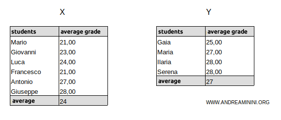
Let’s consider two distributions, X and Y, which represent the grades of two groups of students.

Distribution X has an average grade of 24:
$$ \mu_X = \frac{21+23+24+21+27+28}{6} = \frac{144}{6} = 24 $$
Distribution Y has an average grade of 27:
$$ \mu_Y = \frac{25+27+28+28}{4} = \frac{108}{4} = 27 $$
Next, let’s calculate the standard deviation for both distributions.
Distribution X has a standard deviation of approximately 2.7080:
$$ \sigma_x = \sqrt{ \frac{1}{6} \cdot [ (21- 24)^2 + (23- 24)^2 + (24- 24)^2 + (21- 24)^2 + (27- 24)^2 + (28- 24)^2 ] } $$
$$ \sigma_x = \sqrt{ \frac{1}{6} \cdot [ (-3)^2 + (-1)^2 + (0)^2 + (-3)^2 + (3)^2 + (4)^2 ] } $$
$$ \sigma_x = \sqrt{ \frac{1}{6} \cdot ( 9 + 1 + 0 + 9 + 9 + 16 ) } $$
$$ \sigma_x = \sqrt{ \frac{1}{6} \cdot 44 } $$
$$ \sigma_x = \sqrt{ 7.33333 } $$
$$ \sigma_x = 2.7080 $$
Distribution Y has a standard deviation of approximately 1.2247:
$$ \sigma_y = \sqrt{ \frac{1}{4} \cdot [ (25- 27)^2 + (27- 27)^2 + (28- 27)^2 + (28- 27)^2 ] } $$
$$ \sigma_y = \sqrt{ \frac{1}{4} \cdot [ (2)^2 + (0)^2 + (1)^2 + (1)^2 ] } $$
$$ \sigma_y = \sqrt{ \frac{1}{4} \cdot [ 4 + 0 + 1 + 1 ] } $$
$$ \sigma_y = \sqrt{ \frac{1}{4} \cdot 6 } $$
$$ \sigma_y = \sqrt{ 1.5 } $$
$$ \sigma_y = 1.2247 $$
Now, we have all the information needed to calculate the coefficients of variation for the two distributions:
$$ CV_x = \frac{ \sigma_x }{ \mu_x } = \frac{ 2.7080}{24} = 0.1128 = 11.28% $$
$$ CV_y = \frac{ \sigma_y }{ \mu_y } = \frac{ 1.2247}{27} = 0.0453 = 4.53% $$
Distribution X has a coefficient of variation (CVX) of 11.28%, which is higher than the CVY of 4.53% for distribution Y.
Thus, distribution X exhibits greater relative variability compared to distribution Y.
Additional Notes
Here are some important considerations regarding the coefficient of variation:
- Negative Mean: If the mean is negative, you should use the absolute value when calculating the CV. This is because the CV measures relative variability, and a negative mean would distort the results if not adjusted.
- Zero Mean: When the mean is zero, the CV cannot be calculated because it would involve division by zero, making the index undefined.
- Standard Deviation Exceeds the Mean: If the standard deviation (\( \sigma \)) is greater than the absolute value of the mean, the CV may not be meaningful, as high dispersion compared to a small or near-zero mean can lead to misleading interpretations of variability.
- Z-scores
Z-scores (\( z_i \)) provide an alternative way to compare the variability of different phenomena. They are calculated as: $$
z_i = \frac{x_i - \mu}{\sigma} $$ where \( x_i \) is the observed value, \( \mu \) is the mean, and \( \sigma \) is the standard deviation. Z-scores indicate how far a value \( x_i \) is from the mean, measured in terms of standard deviations. They are often used to standardize data, making it easier to compare distributions with different units or scales, and are closely associated with the normal distribution.
And so on.
