Variability concentration in statistics
Concentration measures the variability of an additive phenomenon. In other words, it shows how much the data is concentrated in a statistical variable X.
Concentration can range between two extremes:
- Maximum concentration
When a single unit contains the entire value of the statistical variable X, the concentration is at its maximum. - Equal distribution
When all units hold the same amount of the characteristic, the concentration is zero, which is known as equal distribution or "zero concentration".
How to measure concentration
If a statistical variable has n quantitative values, I arrange them in non-decreasing order, from smallest to largest.
$$ x_{1},x_{2},...,x_{n} $$
Example. I have a distribution X consisting of 8 values.
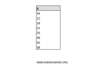
I sort the data in non-decreasing order.
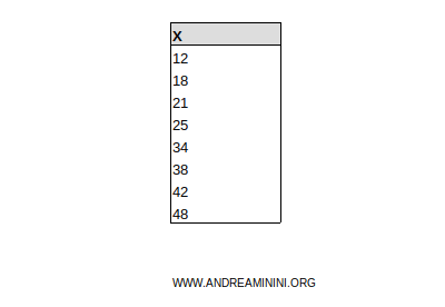
Next, I divide the n observed units into cumulative fractions (pi), which I call cumulative unit fractions.
$$ p_1 = \frac{1}{n} \\ p_2 = \frac{2}{n} \\ \vdots \\ p_n = \frac{n}{n} = 1 $$
Example. In the X distribution, there are n=8 observed units. So, the cumulative unit fractions are: $$ p_1 = \frac{1}{8} = 0.125 \\ p_2 = \frac{2}{8} = 0.25 \\ p_3 = \frac{3}{8} = 0.375 \\ p_4 = \frac{4}{8} = 0.5 \\ p_5 = \frac{5}{8} = 0.625 \\ p_6 = \frac{6}{8} = 0.75 \\ p_7 = \frac{7}{8} = 0.875 \\ p_8 = \frac{8}{8} = 1 $$ I add these to the previous table.
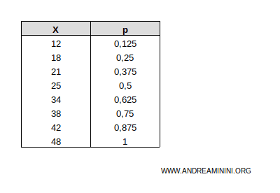
The cumulative unit fractions range from 0 to 1.
I then calculate the total value xtot of the characteristic in the statistical variable.
$$ x_{tot} = \sum_{i=1}^n x_{i} $$
Example. In this case, the total of the observations is xtot=238.
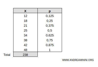
Next, I calculate the cumulative total x' of the observations.
Example. I add the cumulative column x' to the table.
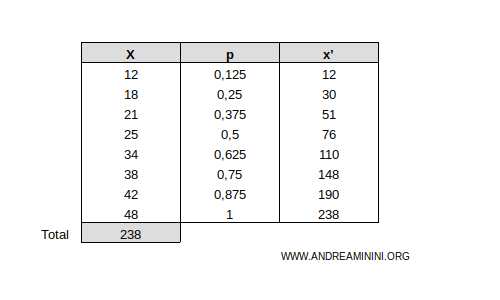
Finally, I calculate the cumulative fractions of the characteristic.
$$ q_1 = \frac{1}{ x_{tot} } \cdot \sum_{i=1}^1 x_i $$
$$ q_2 = \frac{1}{ x_{tot} } \cdot \sum_{i=1}^2 x_i $$
$$ q_n = \frac{1}{ x_{tot} } \cdot \sum_{i=1}^n x_i = 1 $$
These cumulative fractions also range from 0 to 1.
Example. I add the column q of cumulative fractions of the characteristic to the table.
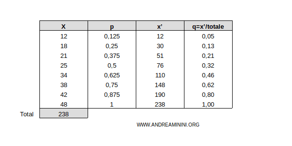
By comparing the cumulative fractions of the observed units (pi) with those of the characteristic (qi), we can visualize the concentration of the data.
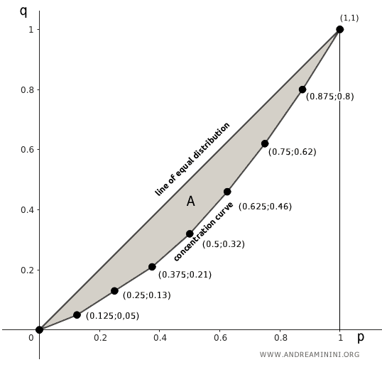
To do this, we use the Lorenz curve or concentration curve.
On the x-axis, we plot the cumulative fractions of the observed units (pi), while on the y-axis, we plot the cumulative fractions of the characteristic (qi).
The diagonal line from the origin (0,0) to the top-right corner (1,1) represents the line of equal distribution.
If the characteristic were evenly distributed, all points would lie on this line.
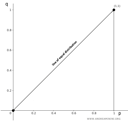
Finally, I plot the points at coordinates (pi,qi) for i=1,...,n.
Connecting these points gives us the concentration curve of the statistical variable.
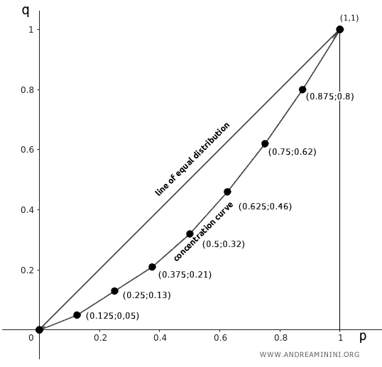
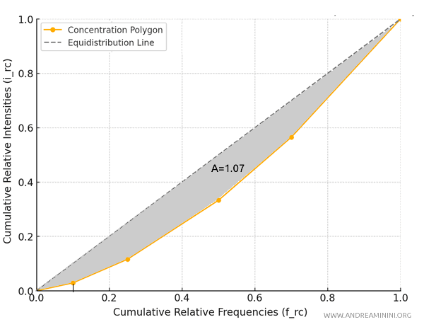
The area between the line of equal distribution and the concentration curve represents the concentration of the statistical variable, known as the concentration area (A).
The concentration index (R) is defined as the ratio between the concentration area (A) and the maximum concentration area.
$$ R = \frac{\text{concentration area (A)}}{\text{maximum concentration area}} $$
This index ranges from 0 to 1, where 1 indicates maximum concentration.
A practical example
Let’s walk through a practical example to calculate the concentration index using a set of values and their frequencies.
Suppose we have a distribution of incomes within a small group of people.
| xi (income) | fi (frequency) |
|---|---|
| 10,000 | 2 |
| 20,000 | 3 |
| 30,000 | 5 |
| 40,000 | 4 |
| 50,000 | 6 |
These values represent the incomes (\( x_i \)) in a group of people, and the corresponding frequencies (\( f_i \)) show how many people receive each income.
We multiply each \( x_i \) by its frequency \( f_i \):
| xi | fi | xi × fi |
|---|---|---|
| 10,000 | 2 | 20,000 |
| 20,000 | 3 | 60,000 |
| 30,000 | 5 | 150,000 |
| 40,000 | 4 | 160,000 |
| 50,000 | 6 | 300,000 |
Next, we calculate the relative frequencies (\( f_i / \sum f_i \)) and add them up to get the cumulative frequencies.
The total of the frequencies (\( \sum f_i \)) is \( 2 + 3 + 5 + 4 + 6 = 20 \).
| xi | fi | Relative frequency (fi/20) | frc | xi × fi | Relative intensity (∑ xi × fi / 690000) | irc |
|---|---|---|---|---|---|---|
| 10,000 | 2 | 0.10 | 0.10 | 20,000 | 0.029 | 0.029 |
| 20,000 | 3 | 0.15 | 0.25 | 60,000 | 0.087 | 0.116 |
| 30,000 | 5 | 0.25 | 0.50 | 150,000 | 0.217 | 0.333 |
| 40,000 | 4 | 0.20 | 0.70 | 160,000 | 0.232 | 0.565 |
| 50,000 | 6 | 0.30 | 1.00 | 300,000 | 0.435 | 1.000 |
The total intensity is 690,000.
$$ 20,000 + 60,000 + 150,000 + 160,000 + 300,000 = 690,000 $$
The cumulative frequencies (\( f_{rc} \)) are the running total of the relative frequencies.
The cumulative relative intensities (\( i_{rc} \)) are the running total of the relative intensities.
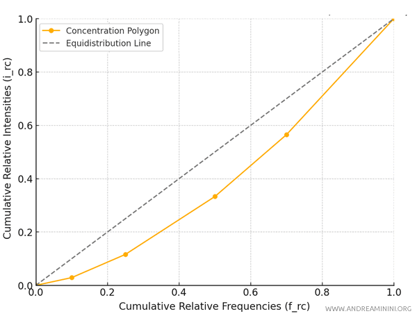
Now, I plot the points \((f_{rc}; i_{rc})\) on a Cartesian plane and connect them to form the concentration curve.
| frc | irc |
|---|---|
| 0.10 | 0.029 |
| 0.25 | 0.116 |
| 0.50 | 0.333 |
| 0.70 | 0.565 |
| 1.00 | 1.000 |
Below is a Cartesian plot that shows the concentration curve alongside the line of equal distribution.
The points represent the cumulative relative frequencies (\( f_{rc} \)) and cumulative relative intensities (\( i_{rc} \)), while the dashed line shows the line of equal distribution.
To calculate the concentration index, I need to find the area between the line of equal distribution (the bisector of the first quadrant, \( y = x \)) and the concentration curve.
The maximum concentration area is always 0.5.
Note. The maximum concentration area is 0.5 because it represents the area of the triangle formed by the line of equal distribution \( y = x \), which depicts a perfectly equal distribution in the plane of cumulative relative frequencies and cumulative relative intensities. This line forms a triangle with the points (0,0), (1,0), and (1,1), where both the base and height are 1. The area of this triangle is calculated as: $$ \text{Area} = \frac{1 \times 1}{2} = 0.5 $$ This area represents the highest possible concentration and is used to normalize the actual concentration area, enabling the calculation of the concentration index \( R \).
To find the concentration area, I calculate the area between the curve and the horizontal axis of the cumulative frequencies.
I break down the area under the curve into triangles and trapezoids based on the curve’s points:
- \( (0.0, 0.0) \)
- \( (0.10, 0.029) \)
- \( (0.25, 0.116) \)
- \( (0.50, 0.333) \)
- \( (0.70, 0.565) \)
- \( (1.00, 1.000) \)
This results in five basic geometric shapes: one triangle and four trapezoids.
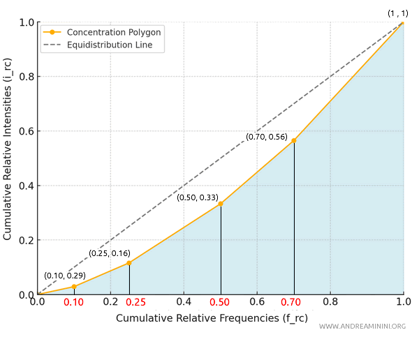
The first segment extends from point \((0, 0)\) to \((0.10, 0.029)\).
This forms a triangle with a base of \( 0.10 - 0.00 = 0.10 \) and a height of \( 0.029 \).
Thus, the area of the initial triangle is:
$$ \text{Area} = 0.5 \times \text{Base} \times \text{Height} = 0.5 \times 0.10 \times 0.029 = 0.00145 $$
For each subsequent segment, I calculate the area of the trapezoid using the formula:
$$ \text{Area} = 0.5 \times (\text{Height}_1 + \text{Height}_2) \times (\text{Base}) $$
The trapezoid between \((0.10, 0.029)\) and \((0.25, 0.116)\) has a base of \( 0.25 - 0.10 = 0.15 \) and heights \( 0.029 \) and \( 0.116 \).
$$ \text{Area} = 0.5 \times (0.029 + 0.116) \times 0.15 = 0.010875 $$
The trapezoid between \((0.25, 0.116)\) and \((0.50, 0.333)\) has a base of \( 0.50 - 0.25 = 0.25 \) and heights \( 0.116 \) and \( 0.333 \).
$$ \text{Area} = 0.5 \times (0.116 + 0.333) \times 0.25 = 0.056875 $$
The trapezoid between \((0.50, 0.333)\) and \((0.70, 0.565)\) has a base of \( 0.70 - 0.50 = 0.20 \) and heights \( 0.333 \) and \( 0.565 \).
$$ \text{Area} = 0.5 \times (0.333 + 0.565) \times 0.20 = 0.089800 $$
The trapezoid between \((0.70, 0.565)\) and \((1.00, 1.000)\) has a base of \( 1.00 - 0.70 = 0.30 \) and heights \( 0.565 \) and \( 1.000 \).
$$ \text{Area} = 0.5 \times (0.565 + 1.000) \times 0.30 = 0.234 $$
Now, I sum the areas of all the trapezoids and the triangle:
$$ \text{Total area} = 0.00145 + 0.010875 + 0.056875 + 0.089800 + 0.234 = 0.393 $$
The total area under the concentration curve, calculated by summing the areas of the individual trapezoids and the triangle, is 0.393.
This value allows me to determine the concentration area by subtracting the curve’s total area (0.393) from the maximum area (0.5):
$$ \text{concentration area} = 0.5 - 0.393 = 0.107 $$
The concentration area is 0.107.
Therefore, the concentration index is calculated as follows:
$$ R = \frac{\text{concentration area}}{\text{maximum concentration area}} = \frac{0.107}{0.5} = 0.214 $$
The concentration index \( R = 0.214 \) suggests that the income distribution within the group is moderately concentrated, equal to 21.4%.
A value closer to 1 indicates higher concentration (unequal distribution), while a value closer to 0 suggests a more even distribution.
And so forth.
