Solving Linear Systems with the Gauss Jordan Method
A linear system can be solved by applying the Gauss Jordan elimination procedure to the augmented matrix A|B associated with the system.
How to Solve a Linear System with Gauss Jordan Elimination
The augmented matrix A|B is reduced to row echelon form by performing Gauss Jordan operations.
Why? A row echelon system is straightforward to handle because each equation isolates one more variable than the previous one, which makes the overall structure easy to read and solve.
By identifying the pivot positions, we can determine the rank of both the coefficient matrix A and the augmented matrix A|B.
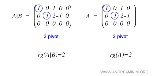
Note. According to Gauss’s rank method, the number of pivot positions in a row echelon matrix is exactly the rank of that matrix.
The ranks of A and A|B allow us to determine whether the system is consistent, thanks to the Rouché Capelli theorem.
If the system is consistent and the coefficient matrix is rectangular, we must assign parameters to the variables corresponding to the non-pivot columns in A.
Note. The final column of the augmented matrix A|B is not parametrized because it represents the constants of the system.
Introducing parameters effectively turns the coefficient matrix into a square system.

At this point, the remaining variables can often be determined directly or, if needed, by applying Cramer’s rule.
A Worked Example
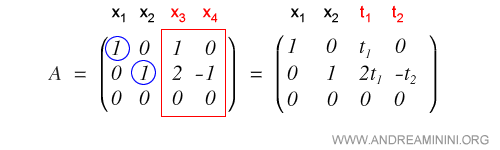
Consider a linear system consisting of three equations in four variables:
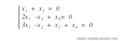
We begin by writing the system in matrix form.
The coefficient matrix is A, while A|B is the corresponding augmented matrix.
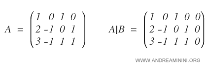
Since A is rectangular, Cramer’s rule does not apply.
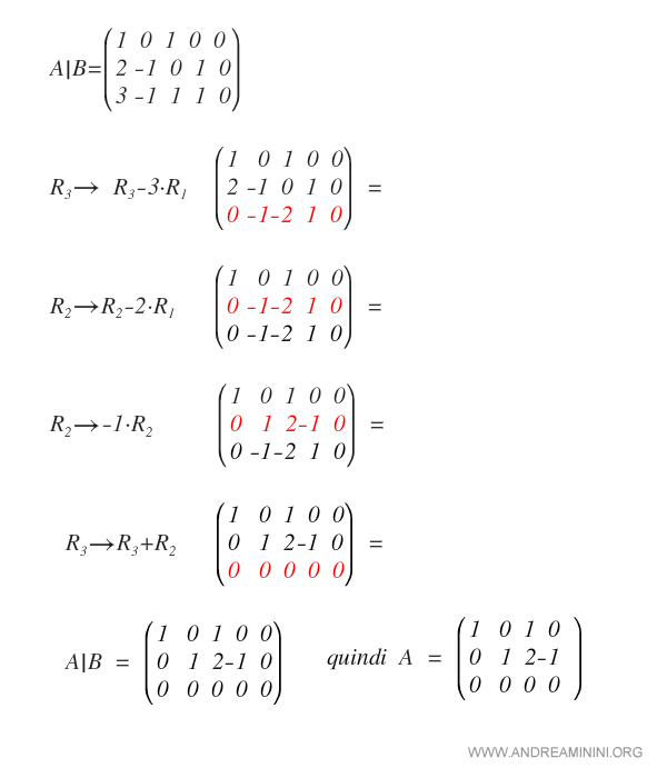
To convert the problem into a square system, we perform Gauss Jordan elimination.
Using Gauss operations, we reduce A|B to row echelon form.
We now compute the rank of A and A|B by counting their pivot positions.

The two matrices have the same rank.
Consequently, by the Rouché Capelli theorem, the system is consistent and admits one or more solutions.
We now parametrize the variables associated with the non-pivot columns of the coefficient matrix.
This yields the first two solutions by setting x1 = t1 and x2 = t2.
We can now rewrite the system accordingly.
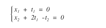
Next we isolate all constant terms on the right-hand side.
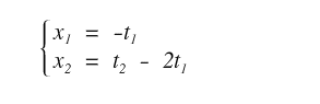
This gives us the remaining variables x3 and x4.
Note. In this particular example, the solutions follow directly from the reduced form. In other cases, once the coefficient matrix has become square, x3 and x4 could be computed using Cramer’s rule.
Including the parametrized variables x1 and x2, the full solution of the system is:
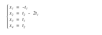
This completes the solution of the system using the Gauss Jordan elimination method.


