Decision Trees

Decision trees are a fundamental concept in machine learning. They are also known as decision tree.

Particularly, decision trees are used in inductive learning processes, those based on observing the surrounding environment.

How a Decision Tree Works

A decision tree is a system with n input variables and m output variables.

The input variables (attributes) are derived from observing the environment. The final output variables, on the other hand, identify the decision/action to be taken.

Note. In very deep decision trees, the intermediate output variables, emerging from parent nodes, coincide with the input variables of the child nodes. These intermediate output variables influence the path towards the final decision.

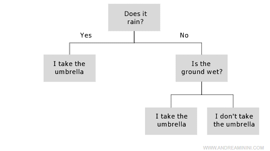
The decision-making process is depicted as an inverted logical tree, where each node is a conditional function.

Each node tests a condition (test) on a particular property of the environment (variable) and has two or more branches downward accordingly.

The process involves a sequence of tests. It always starts from the root node, the parent node at the top of the structure, and proceeds downward.

Depending on the values detected at each node, the flow takes one direction or another, progressively moving downward.

Note. As the selection process continues downward, the hypothesis space narrows because many of the tree's decision branches are eliminated.

The final decision is found in the terminal leaf nodes, at the very bottom.

Thus, after analyzing various conditions, the agent reaches the final decision.

Note. Due to its expressiveness and simplicity, the decision tree representation is also widely used in marketing to construct scripts used by salespeople and telemarketers.

Types of Decision Trees

In a decision tree, variables can be:

• Discrete Variables. Variables have integer numeric values. In these cases, we talk about classification.

  Note. The simplest discrete form is boolean classification where variables have only two values: zero (false) or one (true).

• Continuous Variables. Variables have real numeric values. Between any two real numbers, there's always another intermediate number. In these cases, we refer to regression.

  Note. Representing continuous variables is more complex but better suited to fuzzy logic and logic under conditions of uncertainty, where there's no clear distinction between true and false, between a statement and its negation, etc.

Pros and Cons

Advantages

Logical trees boast the distinct advantage of simplicity. They are easy to understand and execute.

Compared to neural networks, a decision tree is easily comprehensible by humans.

Therefore, humans can verify how the machine arrives at a decision. And possibly disagree.

Example. A decision tree applied in medicine provides diagnoses. Since this is a crucial decision for the patient, it's always advisable for a doctor to verify the classification process that led the machine to that decision. For a human, this is undoubtedly easier with a decision tree than a neural network.

There might be more efficient decision-making criteria, better suited to machine logic but less comprehensible to humans.

This aspect is significant.

Moreover, boolean decision trees are easily developed into programming code, as they can be represented with any propositional language.

Note. All boolean functions can be depicted as a decision tree, and vice versa.

This characteristic is known as the expressiveness of decision trees.

A Practical Example

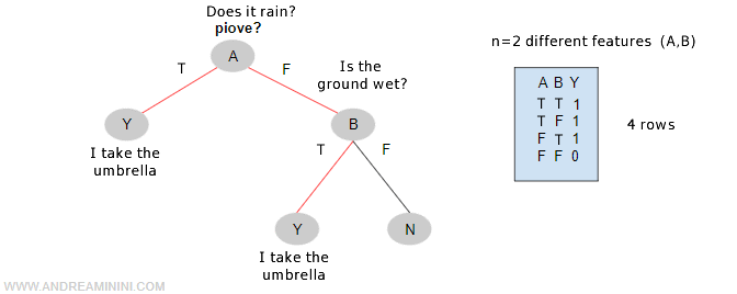
The following tree comprises two attributes or tests (A, B) and a boolean output value (Yes / No) for the function ShouldITakeAnUmbrella(s).

In propositional language, the truth function ShouldITakeAnUmbrella(s) can be written as follows:

The proposition identifies the two possible paths in the decision tree that lead to the terminal node Y from the root, namely the nodes where the function ShouldITakeAnUmbrella is true, i.e., equals 1.

Explanation. For each state (s), the function ShouldITakeAnUmbrella is true if either proposition 1 or proposition 2 is true. A state (s) is a combination of values that the two attributes A and B can take. Each state is a vector that coincides with a particular row in the truth table and with a specific path from the root to a terminal leaf with a positive outcome (Y).

 

Disadvantages

Decision tree representation is less suitable for complex problems, as the hypothesis space becomes too large.

The algorithm's spatial complexity could become prohibitive.

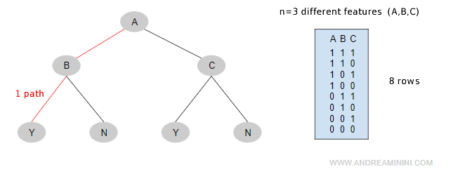
Example. In the simplest case of a boolean tree, for n input attributes (e.g., input variables A, B, C) you need 2ⁿ combinations (paths in the branches) or 2ⁿ rows in a truth table to determine the final decision (Y / N). However, if a node had more attributes (number of classes = number of outgoing branches) or was a non-boolean variable (e.g., temperature), the combinations would be significantly more.

A decision tree can describe only the relationship between a truth function and the logical combinations of attributes. It cannot represent multiple functions.

To do so, another decision tree must be created and associated with the previous one.

Each truth function is a separate decision tree.

Moreover, a decision tree cannot represent all types of functions but only some.

Example. A decision tree cannot represent a function that returns 1 when all attributes are true (parity function) or when the majority of attributes are true (majority functions).