Computing an Inverse Matrix with the Gauss - Jordan Algorithm

In this section, we use the Gauss - Jordan elimination algorithm to compute the inverse matrix A^-1 of an invertible matrix A.

What is the Gauss - Jordan algorithm? It is a systematic procedure for reducing a matrix to row echelon or reduced row echelon form.

How the Gauss - Jordan method finds an inverse

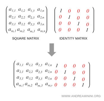
We begin by augmenting the matrix A with the identity matrix, forming the block matrix [A | I].

The algorithm then transforms this augmented matrix into [I | A^-1].

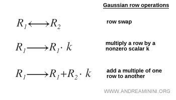
Note. The allowed row operations are: swapping two rows, multiplying a row by a nonzero scalar k, and adding a multiple of one row to another. These can be combined as needed. The Gauss - Jordan algorithm applies them step by step to eliminate all non-pivot entries.

If the left block becomes the identity, then the right block is the inverse matrix of A.

The algorithm specifies the exact sequence of operations to follow, making it ideal for computation.

How does Gauss - Jordan differ from Gaussian elimination? In both cases, the idea is to move the identity matrix from the right to the left to obtain the inverse. With Gaussian elimination, you are free to choose the order of operations, which is convenient for hand calculations. Gauss - Jordan, by contrast, prescribes a fixed sequence of steps, making it better suited for automated computation.

A worked example

Suppose we are given a square matrix A and want to find its inverse A^-1:

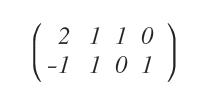
We augment A with the identity matrix I of the same order (2 in this case):

The goal is now to shift the identity to the left using Gaussian row operations.

This produces the first pivot, a 1 on the main diagonal:

Next, we eliminate the entry below the pivot (−1) using the Gauss - Jordan formula.

Here \( q_j \) is the entry to eliminate (−1), \( p_k \) is the pivot (1), and \( R_i \) and \( R_k \) are the row to update and the pivot row, respectively.

The ratio is \( q_j / p_k = -1 \):

Apply \( R_2 - (q_j/p_k)\cdot R_1 \) to every entry of row 2. The factor (−1) is applied uniformly across the row.

This zeros out the column below the pivot. The first column is now complete.

We now move to the second column. The pivot here is 3, which we scale to 1 by multiplying row 2 by 1/3:

This gives the second pivot, the 1 on the second diagonal position:

There remains a nonzero entry above the pivot (2 in the first row). To eliminate it, we apply \( R_1 - (q_j/p_k)\cdot R_2 \). Here \( q_j = 2 \) and \( p_k = 1 \), so the ratio is 2:

Apply the update to row 1:

This eliminates the 2 in the second column.

At this point, the left block is the identity matrix.

Therefore, matrix A is invertible, and the right block is its inverse A^-1:

So the inverse matrix of A is:

To confirm, multiply A by A^-1. The product is the identity I:

Note. I have also solved this example using other methods for computing inverses, and in each case the result was the same.