Euler's Finite Difference Method

What is Euler’s method?

Euler’s method is a numerical technique used to approximate a particular solution of a differential equation, starting from a given initial condition. It’s also referred to as the finite difference method.

What is it used for?

Finding the exact solution to a differential equation can be challenging, especially since many such equations can't be solved analytically.

In practice, however, an approximate solution is often sufficient for modeling real-world phenomena.

To obtain this kind of solution, we can turn to one of the many techniques from numerical analysis. Euler’s method is one of the simplest and most intuitive among them.

Note. Euler’s method does have its limitations: it only yields particular solutions, not the general form of a differential equation. Additionally, it requires an initial condition to get started. For these reasons, it’s especially useful in applied contexts, where we’re interested in solving specific, concrete problems rather than deriving general solutions.

How Euler’s Method Works

The core idea of Euler’s method is to approximate the derivative \( y' \) using the difference quotient \( \Delta y / \Delta x \):

$$ y' \Rightarrow \frac{\Delta y}{\Delta x} $$

A general first-order differential equation can be written as:

$$ y' = f(x, y) $$

The first step is to define an initial condition:

$$ y_0 = y(x_0) $$

To estimate the solution at a target point \( x^* \), we divide the interval \( (x_0, x^*) \) into \( n \) equal subintervals of width \( \Delta x \):

$$ \Delta x = \frac{x^* - x_0}{n} $$

We then compute the approximate values \( y_i \) and the corresponding increments \( \Delta y_i \):

$$ y_i = f(x_i) $$

$$ \Delta y_i = y_{i+1} - y_i $$

Here, \( i \) ranges over the integers from \( 0 \) to \( n \).

Since we’re replacing the derivative with the difference quotient, we write:

$$ \frac{\Delta y}{\Delta x} = y' = f(x, y) $$

which leads to:

$$ \Delta y = f(x, y) \Delta x $$

This gives us a recursive formula for estimating the next value of the function:

$$ y_{i+1} = y_i + f(x_i, y_i) \Delta x $$

Each new value \( y_{i+1} \) is computed from the previous approximation \( y_i \) by adding the estimated change \( \Delta y \):

$$ y_{i+1} = y_i + \Delta y $$

Note. This process can be implemented on a computer using either iteration or recursion. For problems involving a large number of steps, iteration is generally preferred, as it is more memory-efficient than recursion.

Each iteration produces a point \( (x_i, y_i) \) in the Cartesian plane.

Connecting these points with straight-line segments yields a piecewise-linear approximation of the graph of \( y(x) \) over the interval.

A Practical Example

Let’s walk through a concrete example using the first-order differential equation:

$$ y' = y + x $$

This equation was purposely selected because its exact solution is known. This allows us to directly compare the approximate numerical result with the analytical (exact) one.

Note. When working with numerical methods, it's good practice to validate their performance on so-called “toy problems” - scenarios where the analytical solution is known. This helps assess both accuracy and reliability.

Our goal is to estimate the particular solution at the point \( x^* = 1 \):

$$ x^* = 1 $$

We’ll use the initial condition \( x_0 = 0 \), \( y_0 = 1 \):

$$ x_0 = 0 $$

$$ y_0 = y(x_0) = y(0) = 1 $$

This defines our interval of interest: \( (0, 1) \):

$$ (x_0, x^*) = (0, 1) $$

We divide the interval into 5 equal subintervals, each of width \( \Delta x = 0.2 \):

$$ \Delta x = \frac{x^* - x_0}{n} = \frac{1 - 0}{5} = 0.2 $$

We can now proceed with the iteration.

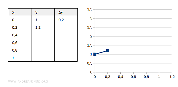
Step 1

We start with the known value at \( x = 0 \):

$$ x_0 = 0 \quad y_0 = 1 $$

Compute the increment:

$$ \Delta y_1 = f(x_0, y_0) \cdot \Delta x $$

$$ = f(0, 1) \cdot 0.2 $$

Given that \( f(x, y) = y + x \):

$$ \Delta y_1 = (1 + 0) \cdot 0.2 = 0.2 $$

The next estimate is:

$$ y_1 = y_0 + \Delta y_1 = 1 + 0.2 = 1.2 $$

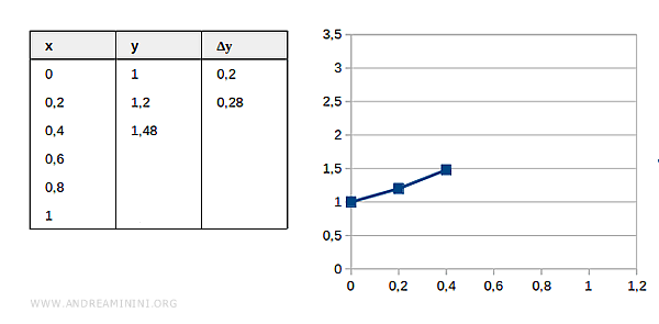
Step 2

Estimated value at \( x = 0.2 \):

$$ x_1 = x_0 + \Delta x = 0.2 \quad y_1 = 1.2 $$

Compute the increment:

$$ \Delta y_2 = f(x_1, y_1) \cdot \Delta x = (0.2 + 1.2) \cdot 0.2 = 0.28 $$

Update the function value:

$$ y_2 = y_1 + \Delta y_2 = 1.2 + 0.28 = 1.48 $$

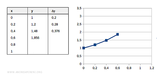
Step 3

Estimated value at \( x = 0.4 \):

$$ x_2 = 0.4 \quad y_2 = 1.48 $$

Compute the increment:

$$ \Delta y_3 = f(x_2, y_2) \cdot \Delta x = (0.4 + 1.48) \cdot 0.2 = 0.376 $$

$$ y_3 = y_2 + \Delta y_3 = 1.48 + 0.376 = 1.856 $$

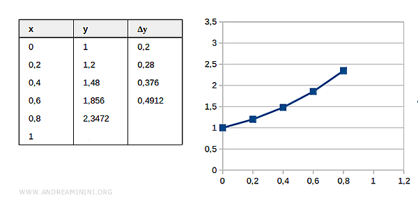
Step 4

Estimated value at \( x = 0.6 \):

$$ x_3 = 0.6 \quad y_3 = 1.856 $$

Compute the increment:

$$ \Delta y_4 = (0.6 + 1.856) \cdot 0.2 = 0.4912 $$

$$ y_4 = 1.856 + 0.4912 = 2.3472 $$

Step 5

Estimated value at \( x = 0.8 \):

$$ x_4 = 0.8 \quad y_4 = 2.3472 $$

Compute the increment:

$$ \Delta y_5 = (0.8 + 2.3472) \cdot 0.2 = 0.62944 $$

$$ y_5 = 2.3472 + 0.62944 = 2.97664 $$

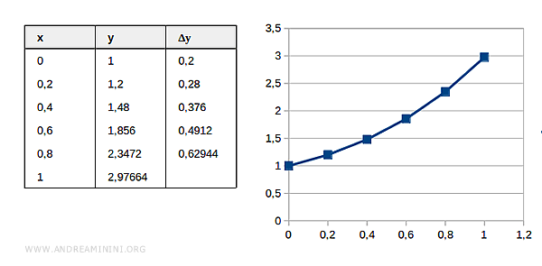
Step 6

Final estimated value at \( x = 1.0 \):

$$ x_5 = 1.0 \quad y_5 = 2.97664 $$

We’ve now reached our target point \( x^* = 1 \).

The resulting approximate solution is:

$$ y(1) = 2.97664 $$

The Euler polygon provides a reasonable approximation of the curve up to \( x = 1 \):

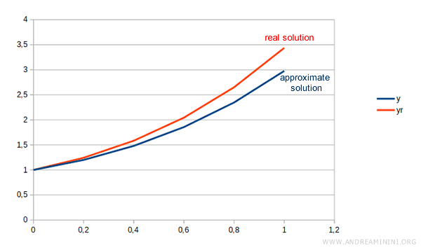
However, the error is still quite significant.

Note. The actual (exact) value at \( x = 1 \) is \( y_R(1) = 3.43 \). The absolute error is:

$$ E = |2.97664 - 3.43| = 0.45 $$

The relative error is:

$$ \frac{E}{y_R} = \frac{0.45}{3.43} \approx 0.131 = 13.1\% $$

An error of 13% is quite substantial.

How can we improve the accuracy?

The simplest way to improve accuracy is to increase the number of subintervals in the partition.

This effectively reduces the step size \( \Delta x \), yielding more precise estimates.

For example, using a partition of 20 intervals:

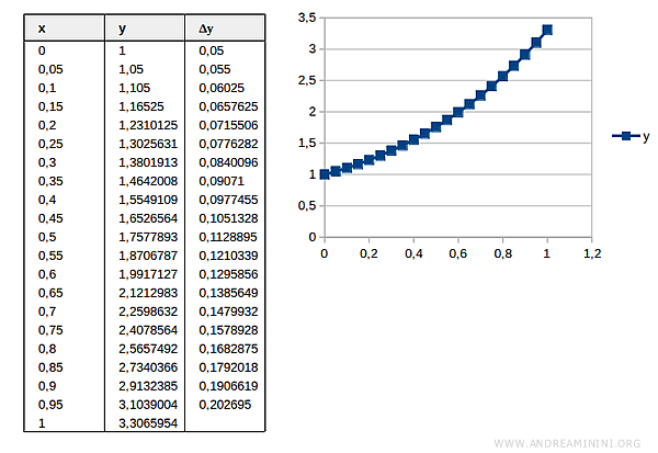
The new estimated value is \( y(1) = 3.30 \), which is much closer to the exact value \( y_R(1) = 3.43 \).

And so on.