Interpolation
Interpolation is a mathematical method used to estimate unknown values within a specific range based on known data points.
In practice, it involves finding a function (called the interpolating function) that passes through or near a set of known data points (called interpolation points or nodes) and using it to predict or estimate the values of other points within that range.
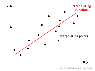
This technique allows us to create a continuous representation of a phenomenon across a given range, even when only a limited set of data points is available.
In simpler terms, interpolation "fills the gaps" between known data points, helping us predict how the phenomenon behaves between the observed points.
Example. If I know only a few reference points within an interval (a,b), interpolation enables me to construct a continuous function that connects them. Once the interpolating function is defined, I can use it to estimate values for points where no direct data is available.
There are two main types of interpolating functions: mathematical interpolation and statistical interpolation, each with its own characteristics and purposes.
- Mathematical interpolation: The interpolating function passes exactly through the data points, useful when the data is precise.
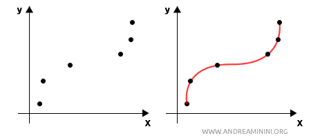
- Statistical interpolation: The interpolating function approximates the data points, minimizing errors, which is useful when the data is subject to noise or measurement errors.
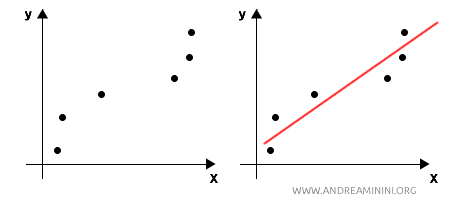
Statistical interpolation is commonly used in statistics and applied sciences, while mathematical interpolation is more often used in theoretical contexts or when the data is considered exact.
Mathematical Interpolation
In mathematical interpolation, the goal is to find an interpolating function that passes exactly through all the known or experimental data points.
In other words, the interpolating function gives the exact values of the known points.
This type of interpolation is used when the data is considered accurate and free from significant errors, or when an exact representation of the phenomenon described by the data is required.
Example
Let’s consider a few interpolation points on a Cartesian plane.
| x | y |
|---|---|
| 1 | 1 |
| 2 | 4 |
| 3 | 9 |
| 4 | 16 |
When I plot the points on the plane, I get a scatter plot where the points are disconnected.
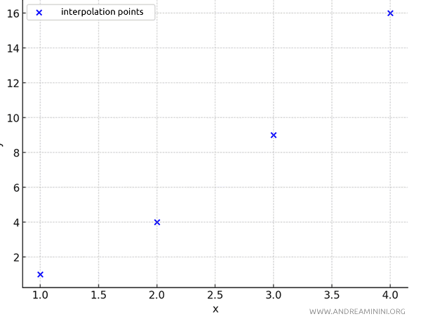
The polynomial function that passes exactly through these points is:
$$ y = x^2 $$
This polynomial perfectly represents the data points, following the rule \(y = x^2\).
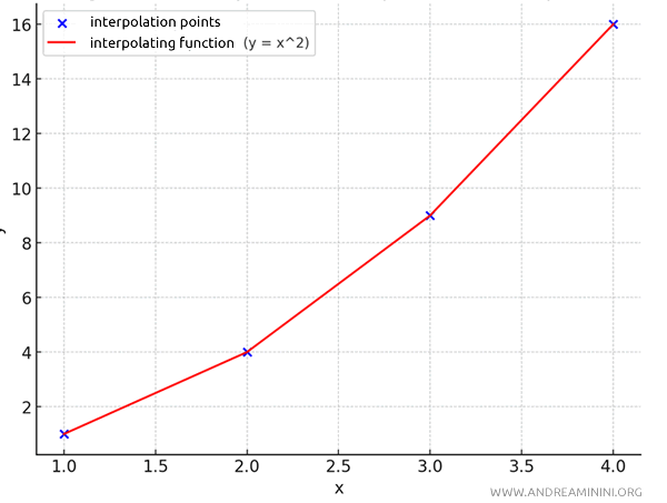
Note. The polynomial \(y = x^2\) was obtained using Lagrange interpolation. In this case, it was straightforward to find the interpolating function. However, this isn’t always the case. Often, finding a mathematical function that passes exactly through all known points can be challenging, which is why statistical interpolation is frequently used.
Statistical Interpolation
In statistical interpolation, the aim is to find a function that gets as close as possible to the known points, minimizing the overall errors between the observed values and those estimated by the interpolating function.
In this case, the interpolating function doesn’t need to pass through each point exactly but should approximate the data points.
This technique is particularly suited for interpreting noisy or uncertain data, such as data from experimental measurements.
Example
Let’s consider the same data as in the previous example.
| x | y |
|---|---|
| 1 | 1 |
| 2 | 4 |
| 3 | 9 |
| 4 | 16 |
This time, however, I want to find a function that comes as close as possible to the data points using statistical interpolation.
The interpolating function doesn’t need to pass through the known points exactly.

To do this, I apply a statistical interpolation technique called linear regression and find a line, $ y = 5x-5 $, that approximates the points (refer to 'calculating the interpolating line').
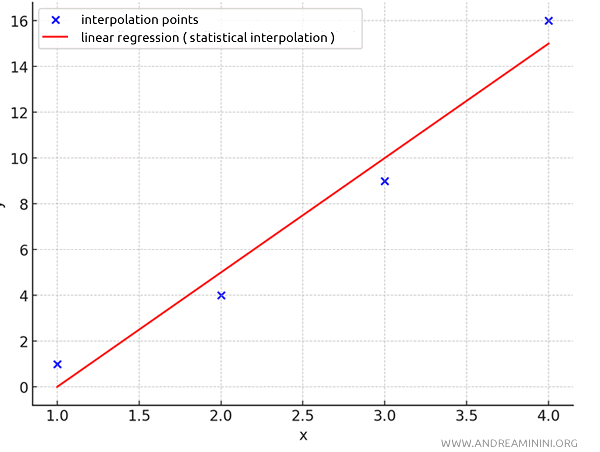
As you can see, the line doesn’t pass exactly through all the points but gets close, minimizing the overall errors. This is a typical example of statistical interpolation.
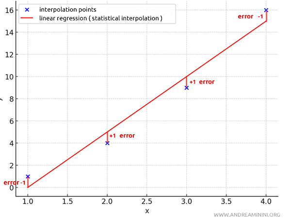
The difference between a known point \( y_i \) and the value estimated by the regression line \( \hat{y}_i \) is called the residual error.
$$ e_i = y_i - \hat{y_i} $$
Where \( y_i \) are the actual values (the known data points), and \( \hat{y}_i \) are the values estimated by the regression line.
| x | y | Estimated values ( $ \hat{y} $ ) | Error $ e_i = y - \hat{y} $ |
|---|---|---|---|
| 1 | 1 | 0.0 | 1.0 |
| 2 | 4 | 5.0 | -1.0 |
| 3 | 9 | 10.0 | -1.0 |
| 4 | 16 | 15.0 | 1.0 |
The sum of the residuals measures the total error in the approximation from interpolation.
$$ e = \sum_{i=1}^{n} e_i = \sum_{i=1}^{n} y_i - \hat{y_i} $$
However, this isn’t a reliable indicator of the total error because, as in this example, the positive and negative residuals can cancel each other out.
$$ e= \sum_{i=1}^{n} y_i - \hat{y}_i = (1-0)+(4-5)+(9-10)+(16-15) $$
$$ e= \sum_{i=1}^{n} y_i - \hat{y}_i = 1-1-1+1 $$
$$ e= \sum_{i=1}^{n} y_i - \hat{y}_i = 0$$
To address this issue, it’s better to calculate the total error using the sum of squared residuals (S).
$$ S = \sum_{i=1}^{n} e_i^2 = \sum_{i=1}^{n} (y_i - \hat{y}_i)^2 $$
This prevents the cancellation between positive and negative residuals.
In this example, the sum of squared residuals (S) is 4.0.
$$ S = \sum_{i=1}^{n} (y_i - \hat{y}_i)^2 = (1-0)^2+(4-5)^2+(9-10)^2+(16-15)^2 $$
$$ S = \sum_{i=1}^{n} (y_i - \hat{y}_i)^2 = (1)^2+(-1)^2+(-1)^2+(1)^2 $$
$$ S = \sum_{i=1}^{n} (y_i - \hat{y}_i)^2 = 1+1+1+1 $$
$$ S = \sum_{i=1}^{n} (y_i - \hat{y}_i)^2 = 4 $$
This value represents the total error in the approximation between the known points and the values estimated by the regression line.
And so on.
