Relative Quadratic Index
The relative quadratic index is a metric used to assess the accuracy of an interpolation or regression model. It’s calculated as the ratio of the standard error (E) to the average of the theoretical values f(x). $$ I = \frac{ E }{\frac{1}{n} \sum_{i=1}^{n} f(x_i)} $$
The standard error (E) is derived as the square root of the mean of the squared differences between the observed values \( y_i \) and the estimated values \( f(x_i) \). Thus, the formula for the relative quadratic index becomes:
$$ I = \frac{\sqrt{\frac{1}{n} \sum_{i=1}^{n} (y_i - f(x_i))^2}}{\frac{1}{n} \sum_{i=1}^{n} f(x_i)} $$
Where \( y_i \) represents the observed values, \( f(x_i) \) are the estimated values from the function, and \( n \) is the number of observations.
This index provides a non-negative value that allows us to compare the model's accuracy in relation to the scale of the data.
It helps determine whether the approximation provided by the function is reasonable when compared to the actual data points.
Note: The closer the index is to zero, the more accurate the approximation. Typically, an index below $ I<0.1 $ is considered acceptable, although the exact threshold may vary based on the context and the required level of accuracy. In some cases, a higher or lower threshold might be more appropriate.
A Practical Example
Let’s look at a dataset $ x $ and $ y $ with $ n=5 $ observations.
| x | y |
|---|---|
| 1 | 2 |
| 2 | 3 |
| 3 | 5 |
| 4 | 4 |
| 5 | 6 |
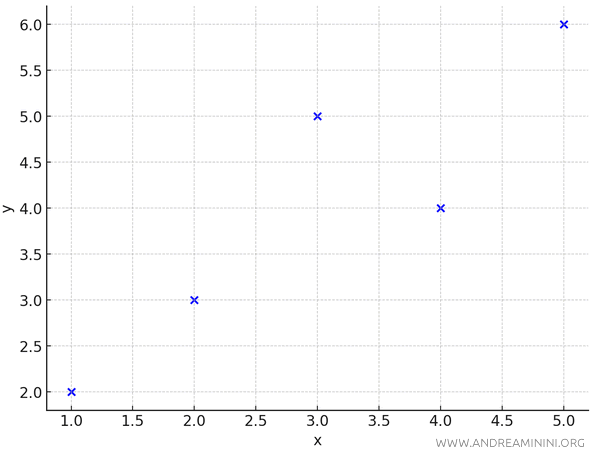
These data points are plotted as scattered points on the Cartesian plane.

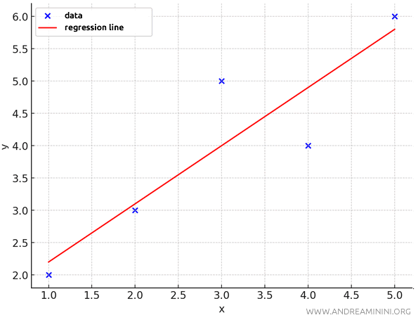
I then calculate an interpolation line \(y = 0.9x + 1.3\) to estimate the intermediate points continuously.

The standard error of interpolation is calculated by examining the partial errors $ e_i = y_i - f(x) $, which represent the differences between the observed values \( y \) and the predicted values \( f(x) \) obtained through the interpolation line \(f(x) = 0.9x + 1.3\).
| x | y | f(x) | e = y - f(x) |
|---|---|---|---|
| 1 | 2 | 2.2 | -0.2 |
| 2 | 3 | 3.1 | -0.1 |
| 3 | 5 | 4.0 | 1.0 |
| 4 | 4 | 4.9 | -0.9 |
| 5 | 6 | 5.8 | 0.2 |
I square the residuals $ e_i^2 = [y_i - f(x)]^2 $ to avoid positive and negative errors canceling each other out.
| x | y | f(x) | e = y - f(x) | e2 |
|---|---|---|---|---|
| 1 | 2 | 2.2 | -0.2 | 0.04 |
| 2 | 3 | 3.1 | -0.1 | 0.01 |
| 3 | 5 | 4.0 | 1.0 | 1.00 |
| 4 | 4 | 4.9 | -0.9 | 0.81 |
| 5 | 6 | 5.8 | 0.2 | 0.04 |
The sum of the squared residuals is 1.90.
$$ \sum_{i=1}^{n} (f(x_i) - \hat{f}(x_i))^2 = \sum_{i=1}^{n} e^2 = 0.04 + 0.01 + 1.00 + 0.81 + 0.04 = 1.90 $$
Therefore, the standard error (E) of the interpolation is:
$$ E = \sqrt{\frac{1}{n} \cdot \sum_{i=1}^{n} (f(x_i) - \hat{f}(x_i))^2} $$
Given that the sum of the squared errors is 1.90 and the number of observations is \(n = 5\).
$$ E = \sqrt{\frac{1}{n} \cdot \underbrace{ \sum_{i=1}^{n} (f(x_i) - \hat{f}(x_i))^2}_{1.90} } $$
$$ E = \sqrt{\frac{1}{5} \cdot 1.90 } $$
$$ E = \sqrt{ 0.38 } $$
$$ E = 0.616 $$
Thus, the standard error is \( 0.616 \).
Now that we have the standard error, we can compute the relative quadratic index.
$$ I = \frac{ E }{\frac{1}{n} \sum_{i=1}^{n} f(x_i)} $$
Substituting E=0.616 and n=5.
$$ I = \frac{ 0.616 }{\frac{1}{n} \sum_{i=1}^{n} f(x_i)} $$
The average of the theoretical values, obtained using the function \(f(x) = 0.9x + 1.3\), is 4.
$$ \frac{1}{n} \sum_{i=1}^{n} f(x_i) = \frac{1}{5} \cdot (2.2+3.1+4.0+4.9+5.8) = \frac{20}{5} = 4 $$
Finally, I substitute the average of the theoretical values into the formula for the relative quadratic index.
$$ I = \frac{ 0.616 }{4} = 0.154 $$
Therefore, in this example, the relative quadratic index of the interpolation is 0.154.
What Are Acceptable Values?
The relative quadratic index \( I \) is always non-negative, as it’s the ratio between two positive quantities: the standard error (a square root) and the mean of the theoretical values, which is conventionally positive.
Thus, the index is always greater than or equal to zero.
$$ I \geq 0 $$
Generally, values close to 0 indicate that the model error is very small relative to the scale of the theoretical values, suggesting the model is highly accurate.
Values greater than 0 suggest a discrepancy between the observed and theoretical values.
The higher the value of \( I \), the greater the relative error.
In practice, specific thresholds are often used to evaluate the model’s accuracy, depending on the context.
For example, a value of \( I \) equal to or less than 0.1 may indicate a very good fit, while higher values might imply the need for model refinement or a more accurate interpolation function.
And so on.
