Least Squares Method

The least squares method allows us to determine the parameters of the best-fitting function by minimizing the sum of squared errors.

In simpler terms, given a set of points (x₁, y₁), (x₂, y₂), and so on, this method finds the slope and intercept of a line $ y = mx + q $ that best fits the data by minimizing the sum of the squared errors.

$$ S = \sum_{i=1}^n e^2_i = \sum_{i=1}^n [y_i - f(x_i)]^2 $$

This approach is commonly used in linear regression to estimate the parameters of a linear function or other types of models that describe relationships between variables.

Note: More generally, this method can be applied to find a curve (instead of a straight line) that best approximates a set of observed data by minimizing the sum of squared differences (vertical distances) between the observed values and those predicted by the model.

How the Least Squares Method Works

Consider a set of points \( (x_i, y_i) \) for \( i = 1, 2, \dots, n \), and our goal is to find the parameters \( m \) and \( q \) that minimize the following objective function:

$$ y = mx + q $$

Where \(y\) is the dependent variable, \(x\) is the independent variable, \(m\) is the slope, and \(q\) is the intercept.

In this case, we're dealing with a linear function, which means it's a straight line.

The parameters \(m\) and \(q\) are chosen to minimize the error, measured as the sum of the squared differences between the observed values \(y_i\) and the predicted values \(y_{\text{predicted}}\).

$$ S(m, q) = \sum_{i=1}^{n} \left( y_i - (mx_i + q) \right)^2 $$

For instance, this method is applied in linear regression.

The first step is to calculate the slope \( m \):

$$ m = \frac{n \sum (x_i y_i) - \sum x_i \sum y_i}{n \sum x_i^2 - (\sum x_i)^2} $$

Where:

• \(n\) is the number of points,
• \(\sum x_i\) is the sum of all \(x\) values,
• \(\sum y_i\) is the sum of all \(y\) values,
• \(\sum x_i^2\) is the sum of the squares of the \(x\) values,
• \(\sum (x_i y_i)\) is the sum of the products of \(x_i\) and \(y_i\). 

Next, we calculate the intercept \( q \):

$$ q = \frac{\sum y_i - m \sum x_i}{n} $$

Once \( m \) and \( q \) are determined, we can write the equation of the regression line.

$$ y = mx + q $$

This is the linear function that best fits the data.

Note: The least squares method can also be extended to polynomial models (curves instead of lines) or more complex models using a more advanced version called generalized least squares.

A Practical Example

Let's walk through a practical example of how the least squares method works for linear regression.

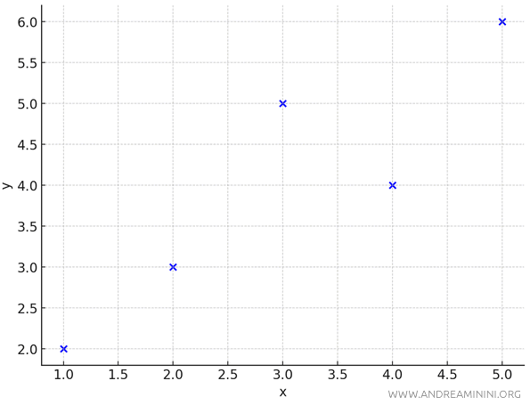
Here are the following experimental data for an independent variable \(x\) and a dependent variable \(y\):

x	y
1	2
2	3
3	5
4	4
5	6

These $ n = 5 $ points are scattered across the plane.

We want to find the regression line \(y = mx + q\) that best fits these points.

To calculate the slope \( m \) of the line, we use the following formula:

$$ m = \frac{n \sum (x_i y_i) - \sum x_i \sum y_i}{n \sum x_i^2 - (\sum x_i)^2} $$

Let’s compute the necessary values:

$$ \sum x_i = 1 + 2 + 3 + 4 + 5 = 15 $$

$$ \sum y_i = 2 + 3 + 5 + 4 + 6 = 20 $$

$$ \sum x_i^2 = 1^2 + 2^2 + 3^2 + 4^2 + 5^2 = 55 $$

$$ \sum (x_i y_i) = (1 \cdot 2) + (2 \cdot 3) + (3 \cdot 5) + (4 \cdot 4) + (5 \cdot 6) = 2 + 6 + 15 + 16 + 30 = 69 $$

Since $ n = 5 $, we substitute these values into the formula for the slope:

$$ m = \frac{n \sum (x_i y_i) - \sum x_i \sum y_i}{n \sum x_i^2 - (\sum x_i)^2} $$

$$ m = \frac{5 \cdot 69 - 15 \cdot 20}{5 \cdot 55 - 15^2} $$

$$ m = \frac{345 - 300}{275 - 225} = \frac{45}{50} $$

$$ m = 0.9 $$

The slope \(m = 0.9\) indicates that for every 1-unit increase in \(x\), \(y\) increases by approximately 0.9 units.

Now, let's calculate the intercept \( q \):

$$ q = \frac{\sum y_i - m \sum x_i}{n} $$

$$ q = \frac{20 - 0.9 \cdot 15}{5} $$

$$ q = \frac{20 - 13.5}{5} $$

$$ q = \frac{6.5}{5} $$

$$ q = 1.3 $$

The intercept \(q = 1.3\) is the value of \(y\) when \(x = 0\).

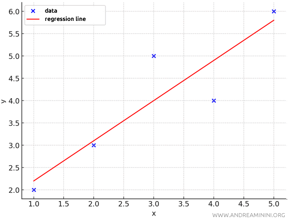
With both the slope \(m = 0.9\) and the intercept \(q = 1.3\) known, we can write the equation of the regression line:

$$ y = mx + q $$

$$ y = 0.9x + 1.3 $$

The line \(y = 0.9x + 1.3\) provides the best linear approximation of the data according to the least squares method.

This line minimizes the sum of the squared errors between the observed values \(y_i\) and the predicted values \(y_{\text{predicted}}\).

x	y	ypredicted	e = y - ypredicted	e2
1	2	2.2	-0.2	0.04
2	3	3.1	-0.1	0.01
3	5	4.0	1.0	1.00
4	4	4.9	-0.9	0.81
5	6	5.8	0.2	0.04

In this case, the sum of the squared errors is:

$$ S(m, q) = \sum_{i=1}^{n} \left( y_i - (mx_i + q) \right)^2 $$

$$ S(0.9, 1.3) = (2-2.2)^2 + (3-3.1)^2 + (5-4)^2 + (4-4.9)^2 + (6-5.8)^2 $$

$$ S(0.9, 1.3) = (-0.2)^2 + (-0.1)^2 + (1.0)^2 + (-0.9)^2 + (0.2)^2 $$

$$ S(0.9, 1.3) = 0.04 + 0.01 + 1.0 + 0.81 + 0.04 $$

$$ S(0.9, 1.3) = 1.9 $$

In conclusion, no other line can further reduce the sum of the squared errors.

And so on.