Standard Error in Interpolation
The standard error (or standard deviation) in interpolation measures the discrepancy between interpolated (estimated) values and actual (observed) values of a function or dataset. $$ E = \sqrt{\frac{1}{n} \cdot \sum_{i=1}^{n} (f(x_i) - \hat{f}(x_i))^2} $$ where \( f(x_i) \) represents the actual values of the function, \( \hat{f}(x_i) \) represents the interpolated values, and \( n \) is the number of data points.
It’s one of the key indicators of interpolation error.
This value represents the average squared deviation between observed values and those estimated through interpolation.
The smaller the standard error, the more accurate the interpolation.
Note. The standard error is used to assess the accuracy of an interpolation method, such as linear, polynomial, or spline interpolation. However, the error may vary depending on the choice of interpolation nodes and the smoothness of the function being interpolated. Also, it doesn’t account for the size of the values being compared. Often, the mean squared error is preferred as an alternative.
A Practical Example
Let’s consider a dataset with $ x $ and $ y $ values:
| x | y |
|---|---|
| 1 | 2 |
| 2 | 3 |
| 3 | 5 |
| 4 | 4 |
| 5 | 6 |
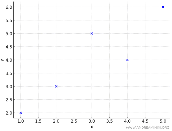
These $ n = 5 $ observed points are scattered across the plane.

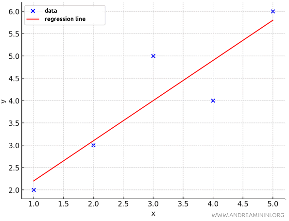
To interpolate them, I’ll use the line \(y = 0.9x + 1.3\).

Now, I want to calculate the standard error of the interpolation.
First, I determine the partial errors $ e_i = y_i - y_{\text{predicted}}(x_i) $, which are the residuals, meaning the difference between the observed values \( y \) and the predicted values \( y_{\text{predicted}} \) based on the line \(y = 0.9x + 1.3\).
This step helps measure how far each data point deviates from the fitted line (interpolation).
| x | y | ypredicted | e = y - ypredicted |
|---|---|---|---|
| 1 | 2 | 2.2 | -0.2 |
| 2 | 3 | 3.1 | -0.1 |
| 3 | 5 | 4.0 | 1.0 |
| 4 | 4 | 4.9 | -0.9 |
| 5 | 6 | 5.8 | 0.2 |
Next, I square the residuals $ e_i^2 = [y_i - y_{\text{predicted}}(x_i)]^2 $ to prevent positive and negative errors from canceling each other out.
| x | y | ypredicted | e = y - ypredicted | e2 |
|---|---|---|---|---|
| 1 | 2 | 2.2 | -0.2 | 0.04 |
| 2 | 3 | 3.1 | -0.1 | 0.01 |
| 3 | 5 | 4.0 | 1.0 | 1.00 |
| 4 | 4 | 4.9 | -0.9 | 0.81 |
| 5 | 6 | 5.8 | 0.2 | 0.04 |
Then, I sum the squared errors to get the total of the partial errors:
$$ \sum_{i=1}^{n} (f(x_i) - \hat{f}(x_i))^2 = \sum_{i=1}^{n} e^2 = 0.04 + 0.01 + 1.00 + 0.81 + 0.04 = 1.90 $$
Now, I can calculate the standard error (E).
$$ E = \sqrt{\frac{1}{n} \cdot \sum_{i=1}^{n} (f(x_i) - \hat{f}(x_i))^2} $$
Given that the sum of the squared errors is 1.90 and the total number of observed points is \(n = 5\).
$$ E = \sqrt{\frac{1}{n} \cdot \underbrace{ \sum_{i=1}^{n} (f(x_i) - \hat{f}(x_i))^2}_{1.90} } $$
$$ E = \sqrt{\frac{1}{5} \cdot 1.90 } $$
$$ E = \sqrt{ 0.38 } $$
$$ E = 0.616 $$
Therefore, the standard error is \( 0.616 \), which represents the average deviation of the points from the predicted values along the regression line.
And that's how it's done.
