Measurement Errors in Physics

Measurement errors refer to the discrepancies between the observed value in a measurement and the actual value of the quantity being measured.

These differences arise from the inherent limitations or imperfections in the instruments or the measurement procedure itself.

They are present in all types of measurements, from basic temperature readings to complex calculations in experimental sciences.

Measurement errors are an unavoidable aspect of scientific measurement, but with careful handling, they can be significantly reduced. For instance, systematic errors require adjustments to instruments or methods, while random errors can be minimized by increasing the number of observations. This approach leads to results that more accurately reflect reality.

Types of Measurement Errors

Measurement errors can be broadly categorized as systematic errors and random errors.

A] Systematic Errors

Systematic errors result from issues with the measurement method or the instrument itself.

They occur consistently in the same direction—either always too high or always too low—every time the measurement is taken.

For instance, if an instrument is improperly calibrated or affected by environmental conditions, it will consistently give a reading different from the true value. This type of error cannot be reduced by taking repeated measurements, as it has a specific and constant cause.

Systematic measurement errors can create an "illusion of precision": they’re particularly deceptive because they recur in the same manner, giving the impression of accuracy when, in reality, the entire measurement process is flawed.

How can systematic errors be managed?

To minimize the impact of systematic errors, I need to regularly calibrate instruments, ensure they’re functioning correctly, and in some cases, use multiple instruments to measure the same quantity.

An effective approach is to compare results from different instruments or methods, or to validate them against reliable reference data, allowing for the identification of any systematic inconsistencies.

B] Random Errors

Random errors are caused by unpredictable, occasional factors, such as slight environmental variations or minor inconsistencies in the measurement process.

Unlike systematic errors, random errors can fluctuate in both directions (either higher or lower) and generally follow a random distribution.

For instance, when timing a heartbeat with a stopwatch, even the slightest delay in pressing the button can influence the result, introducing a random variation with each reading. Similarly, when measuring the length of an object with a ruler, a slight tilt of the instrument can lead to a slightly different result each time. Even room temperature can vary due to a sudden draft or shift in humidity, resulting in fluctuating readings from one measurement to the next.

In some ways, random measurement errors reflect the inherent uncertainty, unpredictability, and randomness of the real world.

They arise from small, uncontrollable factors (e.g., an unexpected vibration, a subtle pressure shift, a fraction of a second difference in human reaction time) and are always present.

Therefore, the best way to handle them is through statistical techniques.

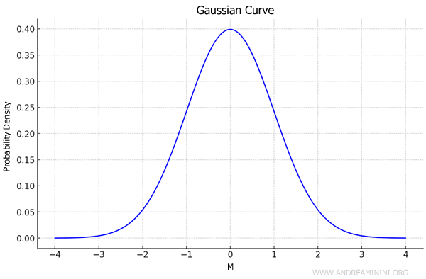
For example, these errors often follow a normal distribution curve, where most results cluster around the average, with extreme values occurring less frequently.

How can random errors be managed?

Since random errors can’t be entirely eliminated, an effective approach to reducing their impact is to increase the number of measurements and calculate their average.

This technique leverages the law of large numbers and the characteristics of the normal distribution.

In other words, by repeating the measurement multiple times, random fluctuations tend to cancel out, and the average result is likely to be closer to the true value.

A Practical Example

I tried timing how long it takes for a pen to fall from a table using a stopwatch, recording five separate results.

Each time, though, I ended up with a slightly different value, likely due to minor reaction-time errors in stopping the stopwatch at just the right moment.

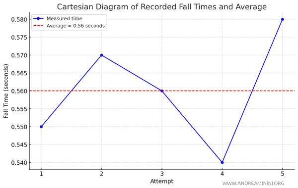
Here are the recorded times, in seconds: 0.55, 0.57, 0.56, 0.54, and 0.58.

Trial	Time (seconds)
1	0.55
2	0.57
3	0.56
4	0.54
5	0.58

These slight differences offer a practical example of random error.

To get a more reliable estimate of the fall time, I calculate the average of the recorded times.

The average is found by adding up all the times and dividing by the total number of measurements, as shown here:

$$ \text{Average} = \frac{0.55 + 0.57 + 0.56 + 0.54 + 0.58}{5} = \frac{2.80}{5} = 0.56 \, \text{seconds} $$

So, the average of 0.56 seconds provides a more dependable estimate of the pen’s actual fall time, as it reduces the impact of random errors in individual measurements.

Example 2

Now, let’s imagine the stopwatch is miscalibrated and runs slightly slow.

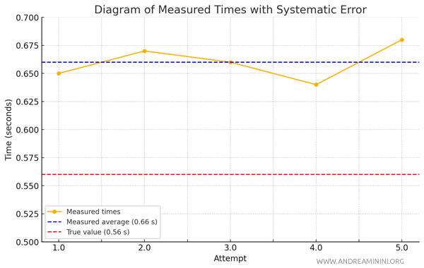
This systematic error leads to an overestimate of the fall time in each measurement.

Here are the recorded times with the miscalibrated stopwatch:

Trial	Time (seconds)
1	0.65
2	0.67
3	0.66
4	0.64
5	0.68

Now, I calculate the average of these readings:

$$ \text{Average} = \frac{0.65 + 0.67 + 0.66 + 0.64 + 0.68}{5} = \frac{3.30}{5} = 0.66 \, \text{seconds} $$

This time, the average comes out to 0.66 seconds—a value consistently higher than the true fall time.

The stopwatch calibration error has skewed all the measurements in the same direction, resulting in values that are all higher than the actual time.

Note: This example demonstrates that a systematic error can’t simply be corrected by averaging; proper calibration of the instrument is needed to obtain accurate measurements.

And so on.