Euler’s Method for Numerical Integration

Euler’s method is a numerical technique for estimating the value of a definite integral of a function $ y = f(t) $ through an iterative process: $$ \int_a^b f(t) \, dt $$ Given an initial condition $ y_0, t_0 $, the method updates the solution using the formula: $$ y_j = y_{j-1} + \frac{dy}{dt}\big|_{t = t_{j-1}} \cdot \Delta t $$ where $ \Delta t $ is the integration step size: $$ t_j = t_{j-1} + \Delta t $$

For a general integral over the interval $[a, b]$:

$$ \int_a^b f(t) \, dt $$

we divide the interval into $ n $ equal parts, yielding a step size:

$$ \Delta t = \frac{b - a}{n} $$

We then choose an initial point $ t_0 $ and evaluate the function at that point:

$$ y_0 = f(0) $$

To approximate the next value, we apply:

$$ y_1 = y_0 + \frac{dy}{dt}\big|_{t = t_0} \cdot \Delta t $$

That is, we multiply the derivative of the function at $ t_0 $ by the step size to obtain an estimate for the value at $ t_1 $.

Note: Since this is an approximation, the result is not exact. The error tends to accumulate progressively over the integration interval.

Explanation

To illustrate the method, we consider the graph of a function $ y = f(t) $ defined over the interval $[a, b]$:

graph of the function y = f(t)

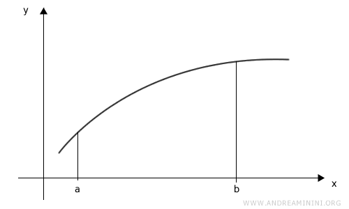
We partition the interval $[a, b]$ into three equal subintervals ($n = 3$):

$$ \Delta x = \frac{b - a}{n} $$

Each subinterval has the same width $ \Delta x $:

partition of the interval [a, b]

Note: For illustrative purposes, we’re using only three intervals. As a result, the final approximation will be fairly rough. Euler’s method becomes more accurate as the number of intervals increases.

We begin with an initial point $ x_0 $, and use the function $ f(x) $ to compute the corresponding value $ y_0 $.

Thus, the starting point of the calculation is $ (x_0, y_0) $:

initial point (x₀, y₀)

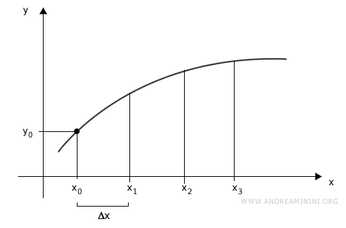
We then compute the next approximation $ (x_1, y_1) $:

$$ \begin{cases} x_1 = x_0 + \Delta x \\\\ y_1 = y_0 + \frac{dy}{dx}\big|_{x = x_0} \cdot \Delta x \end{cases} $$

In this step, we evaluate the derivative at $ x_0 $ - that is, the slope of the tangent line at $ (x_0, y_0) $ - and use it to project a linear estimate reaching $ x_1 $.

This gives us an approximation of the point $ (x_1, y_1) $:

approximate point (x₁, y₁)

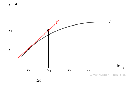
We repeat this process to estimate the next point $ (x_2, y_2) $:

$$ \begin{cases} x_2 = x_1 + \Delta x \\\\ y_2 = y_1 + \frac{dy}{dx}\big|_{x = x_1} \cdot \Delta x \end{cases} $$

This time, we evaluate the derivative at $ x_1 $ and shift the tangent line to pass through the previously computed point $ (x_1, y_1) $.

This yields the next approximation $ (x_2, y_2) $:

approximate point (x₂, y₂)

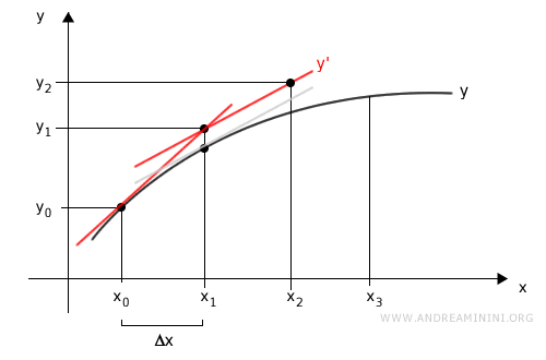
Finally, we perform the same calculations to obtain the last estimate $ (x_3, y_3) $:

$$ \begin{cases} x_3 = x_2 + \Delta x \\\\ y_3 = y_2 + \frac{dy}{dx}\big|_{x = x_2} \cdot \Delta x \end{cases} $$

Once again, we compute the derivative at $ x_2 $ and shift the tangent line through the point $ (x_2, y_2) $ to estimate:

approximate point (x₃, y₃)

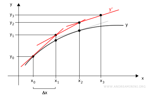
We now have a piecewise linear approximation $ y^* $ to the function $ f(x) $.

This allows us to estimate the area under the curve $ y^* $ and thus approximate the definite integral of $ f(x) $ over the interval $[a, b]$, by summing the areas between: \[ [x_0, x_1],\ [x_1, x_2],\ [x_2, x_3] \].

Since the approximation is linear over each segment, we can compute these areas using basic geometry - rectangles and triangles.

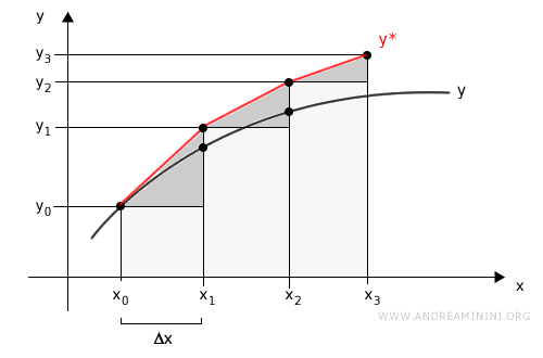
area under the linear approximation

Summing these gives an estimate for the integral of $ f(x) $ over $[a, b]$:

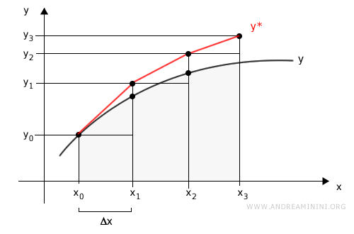
estimated value of the definite integral

And so on.