Uniqueness Theorems for Roots of Functions
Root uniqueness theorems help us determine whether a function has exactly one root in a given interval.
To establish uniqueness, we look at three properties: whether the function is continuous, whether its values at the endpoints have opposite signs, and how its derivatives behave within the interval.
Note. The Intermediate Value Theorem guarantees that a continuous function has at least one root when its values at the endpoints of an interval have opposite signs. However, it does not tell us whether other roots exist. Root uniqueness theorems go a step further by providing conditions that guarantee exactly one root in the interval.
Let's look at two theorems that establish when a root is unique.
First Root Uniqueness Theorem
Let \(f\) be continuous on the closed interval \([a,b]\) and differentiable on the open interval \((a,b)\). If \(f'(x)\neq 0\) for every \(x\in(a,b)\), and \(f(a)\) and \(f(b)\) have opposite signs, then there is exactly one point \(c\in(a,b)\) where the function equals zero: \[ \exists!\,c\in(a,b)\quad\text{such that}\quad f(c)=0. \]
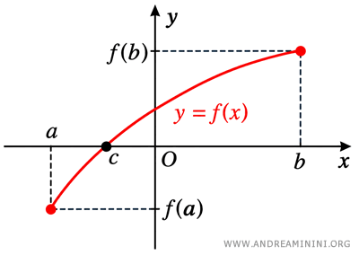
The condition \(f'(x)\neq 0\) means that the derivative never vanishes inside the interval. Since derivatives have the intermediate value property, the derivative cannot change sign without passing through zero. As a result, the function must be strictly increasing or strictly decreasing throughout the interval.
A function that is strictly increasing or strictly decreasing can intersect the x-axis at most once.
Because the function is also continuous and has opposite signs at the endpoints, the Intermediate Value Theorem guarantees that it crosses the x-axis at least once. Combining these two results, we know that the function has exactly one root.
Example
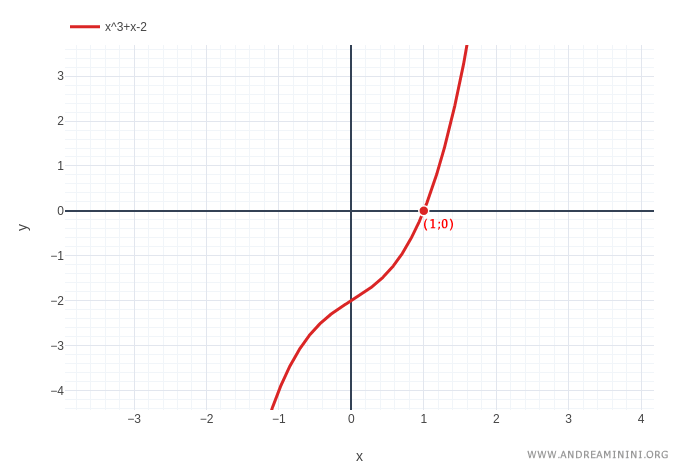
Consider the function below on the interval \( [0,2] \).
\[ f(x)=x^3+x-2 \]
Since this is a polynomial, it is continuous and differentiable throughout the interval.
Its first derivative is
\[ f'(x)=3x^2+1 \]
For every \(x\in(0,2) \), the derivative is strictly positive because \(3x^2\) is nonnegative. Therefore, the derivative never equals zero.
\[ f'(x)=3x^2+1>0 \]
Next, let's evaluate the function at the endpoints:
\[ f(0)=-2<0,\qquad f(2)=8>0 \]
The function takes opposite signs at the endpoints, and its derivative never vanishes inside the interval. Both conditions of the first root uniqueness theorem are satisfied.
Therefore, the function has exactly one root in \((0,2) \). We can find it by substituting \(x=1\), which gives \(f(1)=0 \). Thus, the unique root is \(x=1\).
Proof
We can prove the theorem using proof by contradiction. The idea is to assume that two distinct roots exist and show that this leads to an impossible result.
First, since the function is continuous on \([a,b]\) and takes opposite signs at the endpoints, the Intermediate Value Theorem (Bolzano's Theorem) guarantees that at least one point \(c\in(a,b)\) satisfies
\[ f(c)=0 \]
Now suppose there is another root \(c'\), different from \(c\). Without loss of generality, we can assume that \(c<c'\). This gives us
\[ f(c)=f(c')=0 \]
Consider the smaller interval \([c,c']\). The function is continuous on this interval, differentiable at every interior point, and has equal values at its endpoints.
These are exactly the conditions required by Rolle's Theorem. According to Rolle's Theorem, there must be at least one point \(m\in(c,c')\) where the derivative is zero:
\[ f'(m)=0 \]
But this is impossible. One of the hypotheses of the first root uniqueness theorem states that the derivative is nonzero everywhere in \((a,b)\):
\[ f'(x)\neq 0 \qquad \forall x\in(a,b) \]
Since \((c,c')\subset(a,b)\), the point \(m\) would also lie in \((a,b)\), where the derivative is never zero.
We have reached a contradiction. Therefore, our assumption that two distinct roots exist must be false.
Since the Intermediate Value Theorem guarantees at least one root, and Rolle's Theorem rules out two or more distinct roots, the function must have exactly one root in \((a,b)\).
Note. The two theorems play different roles in the proof. The Intermediate Value Theorem guarantees that a root exists, while Rolle's Theorem shows why a second root cannot exist under the given conditions. Together, they establish both existence and uniqueness.
Second Root Uniqueness Theorem
Let \(f\) be continuous on \([a,b]\) and twice differentiable on \((a,b)\). Suppose that \(f(a)\) and \(f(b)\) have opposite signs, and that the second derivative \(f''(x)\) is either strictly positive for every \(x\in(a,b)\) or strictly negative for every \(x\in(a,b)\). Then there is exactly one point \(c\in(a,b)\) where the function equals zero: \[ \exists!\,c\in(a,b)\quad\text{such that}\quad f(c)=0. \]
This theorem focuses on the second derivative, which tells us about the concavity of the graph.
When \(f''(x)>0\) throughout the interval, the function is strictly convex and its graph is concave up. When \(f''(x)<0\) throughout the interval, the function is strictly concave and its graph is concave down.
Unlike the first theorem, the function does not have to be strictly increasing or strictly decreasing throughout the interval. It may change from decreasing to increasing, or vice versa.
What matters is that the second derivative keeps the same strict sign. Combined with the opposite signs of the function values at the endpoints, this ensures that the graph crosses the x-axis exactly once.
We therefore do not need to determine the sign of the first derivative. Instead, we check that the second derivative is strictly positive everywhere or strictly negative everywhere in the open interval.
Example
Consider the following function on the interval \([0,3]\).
\[ f(x)=x^2-4 \]
Since the function is a polynomial, it is continuous and twice differentiable throughout the interval.
First, we calculate its derivatives:
\[ f'(x)= 2x \]
\[ f''(x)= 2 \]
The second derivative is constant and strictly positive for every \(x\in(0,3)\):
\[ f''(x)=2>0 \]
This tells us that the graph is concave up throughout the interval.
Next, we evaluate the function at the endpoints:
\[ f(0)=-4<0,\qquad f(3)=5>0 \]
The endpoint values have opposite signs, and the second derivative is strictly positive throughout the open interval. Therefore, all the hypotheses of the second root uniqueness theorem are satisfied.
The function must have exactly one root in \((0,3)\). Substituting \(x=2\), we obtain \(f(2)=0\), so the unique root is \(x=2\).
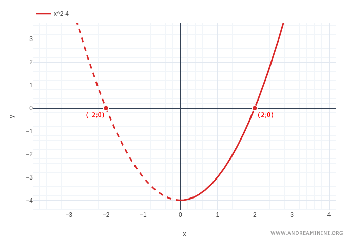
Note. The theorem guarantees that a root is unique only within the interval being considered. It does not mean that the function has no other roots elsewhere. For example, \(f(x)=x^2-4\) has exactly one root in \([0,3]\), but it has two roots, \(x=-2\) and \(x=2\), in the larger interval \([-3,3]\). This does not contradict the theorem. On \([-3,3]\), the function has the same sign at both endpoints, so the opposite-sign condition is not satisfied. The theorem therefore does not apply to that larger interval.
Proof
To make the proof easier to follow, let's start with the case where
\[ f(a)>0,\qquad f(b)<0,\qquad f''(x)>0 \]
The other sign combinations can be handled in much the same way.
Our first assumption is that the second derivative is strictly positive throughout the open interval:
\[ f''(x)>0 \]
Since the second derivative tells us how the first derivative changes, the condition \( f''(x)>0 \) means that the first derivative is strictly increasing throughout the interval.
In terms of the graph, the slope of the tangent line increases as we move from left to right.
To see why the function must have exactly one root, we'll consider three cases.
- First case: the function is strictly increasing.
Suppose the first derivative is strictly positive throughout the interval:
\[ f'(x)>0 \qquad \forall x\in(a,b) \]
This would mean that the function is strictly increasing from \(a\) to \(b\).
However, our initial assumptions tell us that
\[ f(a)>0,\qquad f(b)<0 \]
A strictly increasing function cannot have a positive value at the left endpoint and a negative value at the right endpoint. Its values must increase, not decrease, as \(x\) moves from \(a\) to \(b\).
Therefore, this case is impossible.
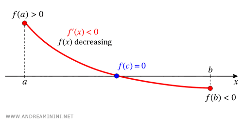
- Second case: the function is strictly decreasing.
Now suppose the first derivative is strictly negative throughout the interval:
\[ f'(x)<0 \qquad \forall x\in(a,b) \]
In this case, the function is strictly decreasing.
We also know that its endpoint values have opposite signs:
\[ f(a) \cdot f(b) < 0 \]
Since the first derivative is negative throughout the interval, it never equals zero:
\[ f'(x)<0 \]
All the conditions of the first root uniqueness theorem are therefore satisfied.
We can conclude that the equation \( f(x)=0 \) has exactly one solution in \((a,b)\).
- Third case: the function decreases and then increases.
Finally, suppose the first derivative equals zero at some point \(m\in(a,b)\):
\[ f'(m)=0 \]
Remember that the first derivative is strictly increasing because \(f''(x)>0\).
This means that the derivative must be negative to the left of \(m\) and positive to the right:
\[ f'(x)<0 \quad \text{for }x<m \]
\[ f'(x)>0 \quad \text{for }x>m \]
As a result, the function is strictly decreasing on \( [a,m] \) and strictly increasing on \( [m,b] \).
The point \(m\) is therefore a minimum.
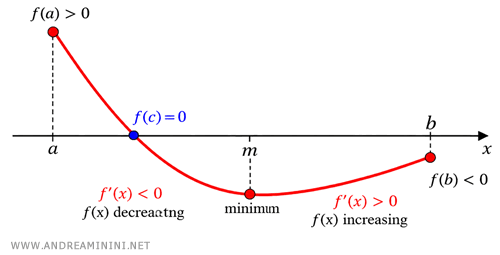
Can this happen if \(f(a)>0\) and \(f(b)<0\)? Yes. After reaching its minimum, the function can start increasing again while remaining below the x-axis.
Let's see why the root is still unique.
Since the function is strictly increasing on \([m,b]\), its value at the minimum must be smaller than its value at the right endpoint:
\[ f(m)<f(b) \]
But we already know that \(f(b)<0\). Combining these inequalities gives
\[ f(m)<f(b)<0 \]
Because the function increases from \(f(m)\) to \(f(b)\), and both values are negative, it remains negative throughout \([m,b]\).
Therefore, there are no roots in \([m,b]\).
We only need to examine the interval \([a,m]\), to the left of the minimum.
Here, the function is strictly decreasing because
\[ f'(x)<0 \]
Its endpoint values also have opposite signs:
\[ f(a)>0,\qquad f(m)<0 \]
All the conditions of the first root uniqueness theorem are satisfied on \([a,m]\).
Therefore, there is exactly one point \(c\in(a,m)\) such that
\[ f(c)=0 \]
Since we have already shown that no roots exist in \([m,b]\), this is also the only root in the entire interval \((a,b)\).
We have now covered all three cases. The first is impossible because it contradicts the endpoint conditions. In the second case, the function is strictly decreasing and has exactly one root. In the third case, the function decreases to a minimum and then increases, but it still crosses the x-axis only once.
Therefore, under the hypotheses of the second root uniqueness theorem, the function has exactly one root in \( (a,b) \):
\[ \exists!\,c\in(a,b):f(c)=0 \]
This completes the proof for the case considered.
The remaining sign combinations can be proved using the same reasoning, with the appropriate changes to the signs and monotonicity.