Bayes’ Theorem

Bayes’ theorem provides a systematic way to compute the probability of a given event A by incorporating available information about another event B. $$ p(A|B) = \frac{ p(A) \cdot p(B|A) }{ p(B) } $$

• p(A|B) and p(B|A) are conditional probabilities (posterior probabilities)
• p(A) and p(B) are marginal probabilities (prior probabilities)

In essence, Bayes’ theorem allows us to evaluate the probability p(A|B) that event A is the underlying cause or explanation of an observed event B.

How does conditional probability work? The conditional probability p(A|B) represents the probability that event A occurs, given that event B has already occurred.

A practical example

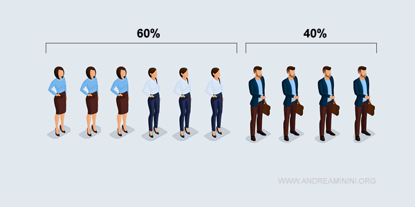
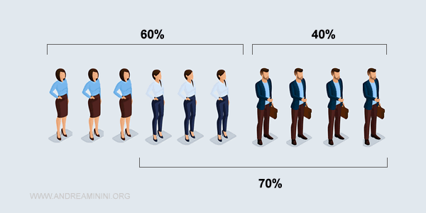
A population is composed of 40% males and 60% females.

All men wear pants, while women wear pants 50% of the time and skirts the other 50% of the time.

An observer sees someone in the distance wearing pants.

What is the probability that this person is female?

The prior probability ( event A ) of the person being female is 60%.

$$ p(A) = 0.6 $$

Note. This is a straightforward estimate based on the population makeup, but it’s not precise enough to answer the question reliably.

The prior probability that a person is wearing pants ( event B ) is 70%.

$$ p(B) = 0.7 $$

Note. All men wear pants (40% of the population), and half of the women do (30%). Therefore, 70% of the population wears pants.

According to the data, the conditional probability (posterior) that a woman (event A) is wearing pants (event B) is 50%.

$$ p(B|A) = 0.5 $$

Note. Half of the women in the population wear pants. This 50% refers only to the female population, not the total population.

Now, we can apply Bayes' Theorem to calculate the probability that the person wearing pants (event B) is female (event A).

$$ p(A|B) = \frac{ p(A) \cdot p(B|A) }{ p(B) } $$

By substituting the known probabilities, we can solve the problem.

$$ p(A|B) = \frac{ 0.6 \cdot 0.5 }{ 0.7 } $$

$$ p(A|B) = 0.43 $$

So, there is a 43% chance that the person observed from a distance is female.

This is the conditional probability of event A (female), given the information we have about event B (pants).

Note. Initially, the prior probability p(A) of the person being female was 60%. The conditional probability, however, is reduced to 43%, which is more accurate because it incorporates the additional information from event B.

This is a simple example of how Bayes' Theorem can be applied in practice.

Derivation

To derive Bayes’ theorem, we start from the definition of conditional probability.

$$ p(E_i \mid E)=\frac{p(E_i \cap E)}{p(E)} $$

In this expression, the quantities \( p(E_i \cap E) \) and \( p(E) \) are not directly known. They must therefore be rewritten in terms of probabilities that are known or can be specified.

From the definition of conditional probability, the probability of the intersection \( E_i \cap E \) can be written as:

$$ p(E\cap E_i)=p(E_i)\,p(E\mid E_i) $$

This provides the first essential component.

We now substitute \( p(E_i \cap E) \) into the original formula:

$$ p(E_i \mid E)=\frac{p(E_i \cap E)}{p(E)} = \frac{p(E_i)\,p(E\mid E_i)}{p(E)} $$

Up to this point, the derivation consists entirely of algebraic manipulations based on the definition of conditional probability.

At this stage, we have already obtained the formal identity underlying Bayes’ theorem. However, the formula is not yet operational, because the probability \( p(E) \) remains unknown and therefore cannot be evaluated directly.

To make the formula usable in actual calculations, it is necessary to express \( p(E) \) in terms of known events.

We therefore apply the decomposition of an event with respect to a partition and rewrite the event \( E \) as the union of pairwise mutually exclusive events.

Since \( E_1, E_2, \dots, E_n \) form a partition of the sample space, the following identity holds:

$$ E=(E\cap E_1)\cup(E\cap E_2)\cup\dots\cup(E\cap E_n) $$

Because these events are mutually exclusive, their probabilities can be summed:

$$ p(E)=p(E\cap E_1)+p(E\cap E_2)+\dots+p(E\cap E_n) $$

Substituting each intersection as before yields:

$$ p(E)=p(E_1)p(E\mid E_1)+p(E_2)p(E\mid E_2)+\dots+p(E_n)p(E\mid E_n) $$

This expression is known as the law of total probability.

We now return to the conditional probability formula \( p(E_i \mid E)  \) and replace \( p(E) \) with the total probability:

$$ p(E_i \mid E)=\frac{p(E_i)\,p(E\mid E_i)}{p(E)} $$

$$ p(E_i \mid E)=\frac{p(E_i)\,p(E\mid E_i)}{p(E_1)p(E\mid E_1)+\dots+p(E_n)p(E\mid E_n)} $$

This is Bayes’ theorem in its operational form.

It is described as operational because all the probabilities appearing in the numerator and denominator are known or specified, with the sole exception of the probability \( p(E_i \mid E) \), which is precisely the quantity to be determined.

In this way, the formula provides a direct and systematic procedure for computing the posterior probability.

Note. Bayes’ theorem does not introduce a new principle in probability theory. It follows directly from the definition of conditional probability, the notion of a partition of the sample space, and the additivity of probability for mutually exclusive events. The use of event decomposition with respect to a partition is what allows the probability of the observed event to be expressed explicitly and makes the theorem genuinely applicable to practical problems.

And so on.