Random Variables

A random variable X is a variable that can take on a random value from a sample space S.

A random variable can assume any value within the sample space.

In other words, it’s a function that maps a random outcome from a set (the sample space) to a variable.

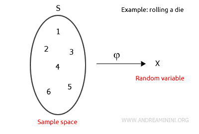
Each outcome has a certain probability of occurring, which may be equal to or different from the others.

Outcomes are mutually exclusive, meaning the occurrence of one excludes the others.

Example. Rolling a die is one of the simplest examples of a random variable. There are six possible outcomes S={1,2,3,4,5,6}, one for each face of the die. It’s considered random because when you roll the die, you can’t predict which face will appear. Whichever face does appear (e.g., 2) prevents the others from occurring, as a die can only show one face at a time.

Thus, the sum of the probabilities of all outcomes is always 1.

The set of all probabilities within the event space is called the probability distribution of the random variable.

Why do we use random variables?

Random variables are typically used to represent the outcome of an experiment where there is uncertainty (a random phenomenon).

Example. You can use a random variable to study the result of rolling dice, drawing a card from a deck, the motion of an electron around an atom’s nucleus, and so on.

A practical example

Example 1

The random variable X represents the outcome of rolling a die.

The sample space S consists of six outcomes, one for each face of the die.

$$ S=\{ 1 \ , \ 2 \ , \ 3 \ , \ 4 \ , \ 5 \ , \ 6 \ \} $$

The random variable can take on any of the values in set S.

Therefore, X can assume an integer value between 1 and 6.

For example, X=3 or X=5, and so on.

$$ X = \begin{cases} 1 \\ 2 \\ 3 \\ 4 \\ 5 \\ 6 \end{cases} $$

Each outcome has a certain probability of occurring.

For instance, the probability of rolling X=3 is:

$$ p(X=3) = \frac{1}{6} $$

Note. Technically, I should write the outcome of the experiment in braces because it’s an element of a set: $$ p(X=\{ 3 \}) = \frac{1}{6} $$ However, for simplicity, we often use the notation without braces: $$ p(X=3) = \frac{1}{6} $$

In this example, each outcome has an equal probability of occurring.

This isn’t always the case.

$$ p(X=1) = \frac{1}{6} \\ p(X=2) = \frac{1}{6} \\ p(X=3) = \frac{1}{6} \\ p(X=4) = \frac{1}{6} \\ p(X=5) = \frac{1}{6} \\ p(X=6) = \frac{1}{6} $$

Since the random variable can take any of these values {1,2,3,4,5,6}, the sum of the probabilities of the outcomes is equal to 1.

$$ p(X=1) + p(X=2) + p(X=3) + p(X=4) + p(X=5) + p(X=6) = $$

$$ = \frac{1}{6} + \frac{1}{6} + \frac{1}{6} + \frac{1}{6} + \frac{1}{6} + \frac{1}{6} = $$

$$ = \frac{6}{6} = 1 $$

In other words, one of the outcomes in the set S={1,2,3,4,5,6} will definitely occur.

Example 2

In this example, the random variable X represents the sum obtained by rolling two dice.

The sample space S consists of 36 possible outcomes:

$$ S = \{ \ (1;1) \ , \ (2;1) \ , \ (3;1) \ , \ ... , \ (6;6) \ \} $$

Note. The pair of values (i;j) represents the result of the first die (i) and the second die (j), separated by a semicolon.

The random variable X can take on an integer value between 2 and 12, which is the sum of the two dice.

In this case, the probabilities for each outcome differ.

This is the probability distribution of the random variable.

$$ P(X=2) = P(\{(1;1)\}) = \frac{1}{36} $$

$$ P(X=3) = P(\{(2;1),(1;2)\}) = \frac{2}{36} $$

$$ P(X=4) = P(\{(3;1),(1;3),(2;2)\}) = \frac{3}{36} $$

$$ P(X=5) = P(\{(4;1),(1;4),(3;2),(2;3)\}) = \frac{4}{36} $$

$$ P(X=6) = P(\{(5;1),(1;5),(3;3),(4;2),(2;4)\}) = \frac{5}{36} $$

$$ P(X=7) = P(\{(6;1),(1;6),(5;2),(2;5),(4;3),(3;4)\}) = \frac{6}{36} $$

$$ P(X=8) = P(\{(6;2),(2;6),(5;3),(3;5),(4;4)\}) = \frac{5}{36} $$

$$ P(X=9) = P(\{(6;3),(3;6),(5;4),(4;5)\}) = \frac{4}{36} $$

$$ P(X=10) = P(\{(6;4),(4;6),(5;5)\}) = \frac{3}{36} $$

$$ P(X=11) = P(\{(6;5),(5;6)\}) = \frac{2}{36} $$

$$ P(X=12) = P(\{(6;6)\}) = \frac{1}{36} $$

Note. The probability of rolling a sum of 7 is much higher than rolling a 12 or a 2.

Again, since the random variable can take on any value between 2 and 12, the sum of the probabilities of all outcomes is equal to 1.

$$ p(\cup^{12}_{i=2} \ X=i \ ) = 1 $$

The Distribution of a Random Variable

The set of probabilities p(X=i) for the events/outcomes of a random variable is known as the distribution or law of the random variable.

Probability distributions of random variables are often represented on a Cartesian graph or as a histogram.

Example

The random variable X represents the sum obtained by rolling two dice.

The sample space S consists of 36 outcomes:

$$ S = \{ \ (1;1) \ , \ (2;1) \ , \ (3;1) \ , \ ... , \ (6;6) \ \} $$

Note. Each outcome is a pair of integers (i,j) representing the result of the first die (i) and the second die (j).

There are 11 possible events in this experiment.

Each event represents the sum of the two dice.

$$ X = \{ 2 \ , \ 3 \ , \ 4 \ , \ 5 \ , \ 6 \ , \ 7 \ , \ 8 \ , \ 9 \ , \ 10 \ , \ 11 \ , \ 12 \} $$

The probability distribution for each event is as follows:

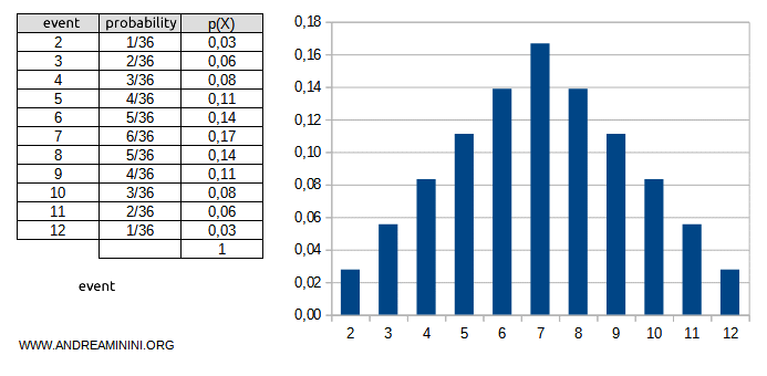
The sum of all probabilities in the distribution is equal to 1.

The difference between an event and an outcome. Typically, I use the term event to refer to a subset of outcomes, distinguishing individual outcomes from groups. For instance, rolling two dice results in 36 possible outcomes S={(1;2),(2;1),...,(6;6)}. The event X is the sum of the two dice. The event X=2 only occurs when the outcome is (1;1), so the probability of this event is P(X)=1/36=0.03. The event X=3 happens when either (1;2) or (2;1) occurs, so the probability p(X=3) =2/36=0.06 represents two out of thirty-six outcomes. And so on.

Types of Random Variables

Random variables can be:

• Discrete Random Variables
  if the sample space contains a finite number of possible values
• Continuous Random Variables
  if the sample space contains an infinite number of possible values

Note. In the case of discrete random variables, the function p(X=k), which assigns a probability to each possible value of X, is called the probability mass function. For continuous random variables, the function p(a<X<b), which assigns a probability to each interval (a;b) of values of X, is called the probability density function.

Example 1

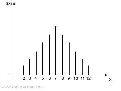
A discrete random variable can take on a finite number of values.

For instance, the sum obtained from rolling two dice.

The function that assigns a probability to each event is called the probability mass function.

 

Example 2

A continuous random variable can take on infinitely many real values.

Its probability distribution is a continuous function f(x).

The function that assigns a probability to each interval (a;b) is called the probability density function.

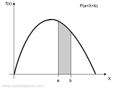
The probability density function is the integral of the function over the interval (a;b)

$$ P(a<X<b) = \int_a^b f(x) \ dx $$

Since the random variable can take any value from the infinite set, if we consider the interval of all real numbers (-∞,∞), the integral of the density function equals 1.

$$ P(-\infty<X<\infty) = \int_{-\infty}^{+\infty} f(x) \ dx = 1 $$

On the other hand, if we consider a single real value (k), the integral equals the probability p(X=k) that the random variable X takes on the value k.

$$ P(X=k) = \int_{k}^{k} f(x) \ dx $$

The Cumulative Distribution Function

The cumulative distribution function represents the probability that the random variable takes on a value less than or greater than a given threshold k. $$ F(X) = p(X<k) $$

To indicate that F is the cumulative distribution function of X, we write

$$ X \sim F $$

Example

The probability that a die roll shows a value less than 4.

$$ F(X)=p(X<4) $$

This occurs when one of the following outcomes happens: 1, 2, or 3.

$$ F(X)=p(X<4)=p(X=1)+p(X=2)+p(X=3) $$

$$ F(X)=p(X<4)=\frac{1}{6}+\frac{1}{6}+\frac{1}{6} $$

$$ F(X)=p(X<4)=\frac{3}{6} $$

$$ F(X)=p(X<4)=\frac{1}{2} $$

So, in this case, the cumulative distribution function gives a 50% probability.

And so on.