Level Curves
Level curves of a function of two variables z = f(x, y) are the set of points (x, y) in the plane that satisfy the equation f(x, y) = k, where k represents a constant output value - either a height or a depth - on the z-axis: $$ \{ \ (x,y) \in \mathbb{R}^2 \ | \ f(x,y)=k \ \} $$
Each level curve corresponds to a horizontal slice of the surface defined by z = f(x, y).

They provide a simplified, intuitive way to visualize functions of two or more variables.
Constructing Level Curves
Begin with the 3D graph of a two-variable function z = f(x, y).
To find a level curve for a given value k, intersect the surface with a horizontal plane at height z = k.
Next, project the resulting intersection onto the xy-plane.
This projection is the level curve at height k. All level curves are drawn in the xy-plane.
By repeating this process for different values of k, we generate additional level curves.
These curves offer a powerful way to analyze the behavior of a function using a two-dimensional representation.
A Practical Example
Consider the function of two variables:
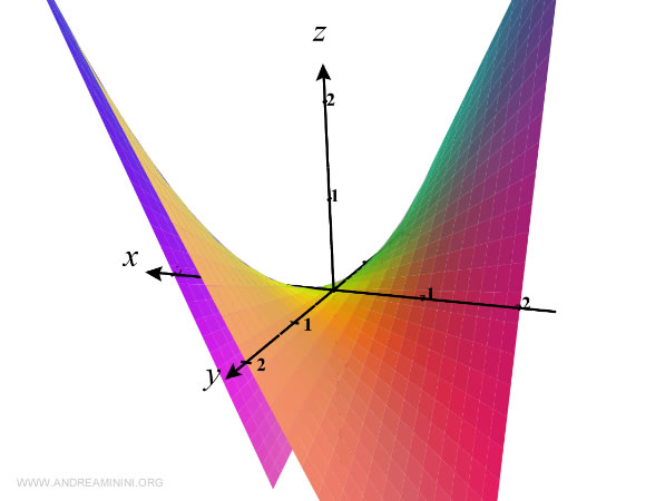
$$ z= f(x,y)=x^2+y^2 $$
Its graph in three-dimensional space is shown below:
We now derive its level curves by solving:
$$ x^2 + y^2 = k $$
No level curves exist for k < 0, since the function only produces non-negative values.
The level curve for k = 0 is simply the point at the origin, (0,0).
For k = 1, we get a circle of radius 1:
$$ x^2 + y^2 = 1 $$
This corresponds to a horizontal slice of the surface at z = 1.
For k = 2, the result is another circle, this time with radius √2:
$$ x^2 + y^2 = 2 $$
Another level curve is added to the xy-plane.
And so on for k = 3, 4, and beyond.
Note. In this example, the level curves get closer together as the value of k increases. When the height increments are uniform but the curves become denser, it indicates a steeper slope on the surface.
Example 2
Let’s take a look at a slightly more complex function:
z = f(x, y) = xy
Its level curves are defined by:
$$ \{ \ (x,y) \in \mathbb{R}^2 \ | \ xy = k \ \} $$
This function is harder to sketch in 3D by hand.
To make it easier to analyze, we use level curves for various positive (z > 0) and negative (z < 0) values of k.
The level curve for k = 0 satisfies:
$$ f(x,y) = x \cdot y = 0 $$
This k = 0 curve consists of the x- and y-axes.
Level curves for k > 0 are rectangular hyperbolas located in the first and third quadrants (positive values).
Level curves for k < 0 are hyperbolas in the second and fourth quadrants (negative values).
Since all level curves are drawn on the xy-plane, it’s easy to confuse them if not clearly labeled.
That’s why each curve should be tagged with its corresponding value of k.
Note. When plotting many level curves, using distinct colors and including a legend helps avoid confusion.
Level Curves and the Gradient
The gradient is always perpendicular to a level curve at the point of calculation. It points in the direction of steepest increase of the function, and its magnitude indicates the rate of change.
Level curves of a function \( f(x, y) \) are the contours in the xy-plane where the function maintains a constant value:
\[ \text{Level curve at } c: \quad f(x, y) = c \]
The closer the curves are to each other, the more rapidly the function changes in that area.
The gradient of a scalar function \( f(x, y) \) is a vector that points in the direction of steepest ascent and is defined by the partial derivatives:
\[ \nabla f(x, y) = \left( \frac{\partial f}{\partial x}, \frac{\partial f}{\partial y} \right) \]
The gradient is orthogonal to the level curve at each point and points toward increasing values of the function. Its magnitude represents how quickly the function is changing at that point.
Example
Let’s revisit the level curves of the function \( f(x,y) = xy \) from earlier.
Along the coordinate axes, the function evaluates to k = 0.
Here, the gradient is perpendicular to the axes and points into the first and third quadrants, where the function increases.
For level curves at k = 1 or k = 2, the gradient remains perpendicular to the curves and continues to point in the direction of maximum increase.
When k = -1 or k = -2, the function takes negative values. These (red) curves lie in the regions where the function decreases.
Even so, the gradient still points toward the direction of growth.
Following a path that crosses level curves means moving through regions where the function is changing. The gradient captures both the direction and the rate of that change.
And so on.


