Maximum and Minimum Points in Multivariable Functions

For functions of two or more variables, local extrema (maximum and minimum points) can occur at:

• Stationary points. Points where the first partial derivatives vanish: \[ \frac{\partial f}{\partial x} = 0 \quad \text{and} \quad \frac{\partial f}{\partial y} = 0 \] These are usually the primary candidates.
• Singular points. Points where the function or its derivatives fail to exist - such as at holes, cusps, or corners. Ideally, we avoid these cases, as they make the analysis much more complicated.
• Boundary points. If the domain is bounded (for instance, inside a circle or a square), we also need to examine what happens along the boundary, since extrema could occur right at the edges.

Note. The procedure for identifying local minima and maxima closely parallels the approach used for single-variable functions. For functions of one variable, \( y = f(x) \), extrema occur at stationary points, singular points, and at the endpoints of a closed interval \([a,b]\). In functions of two variables, \( z = f(x,y) \), extrema are found at stationary points, singular points, and along the boundary of the domain, which typically consists of closed curves, such as the circumference of a circle.

By the Weierstrass theorem, if a function of two or more variables is continuous on a compact set (that is, a set that is closed and bounded), then it necessarily attains both an absolute maximum and an absolute minimum on that set.

In other words, there exist points within the domain where the function achieves its greatest and least values.

Note. The Weierstrass theorem provides a sufficient, but not necessary, condition for the existence of absolute extrema. Thus, even if the function is not continuous or the hypotheses of the theorem are not satisfied, it may still possess points where it attains an absolute maximum or minimum.

A Practical Example

Consider the following function defined over the region \( x^2 + y^2 \leq 1 \):

\[ f(x,y) = x^2 + y^2 \]

In other words, we're looking for the extrema of the function inside a circle of radius 1 centered at the origin.

The partial derivatives are:

$$ \frac{ \partial f }{ \partial x}   = 2x $$

$$ \frac{ \partial f }{ \partial y} = 2y $$

Setting the partial derivatives equal to zero yields the system:

$$ \begin{cases}  2x=0 \\ \\ 2y=0 \end{cases} $$

$$ \begin{cases}  x=0 \\ \\ y=0 \end{cases} $$

Thus, there is a single stationary point at the origin \((0,0)\).

This point is clearly a local minimum, since \( f(0,0) = 0^2+0^2 = 0 \), and the function can only take on non-negative values. Consequently, it cannot achieve values lower than zero.

We must also check for the presence of singular points and investigate the boundary.

In this case, there are no singular points inside the domain (the interior of the circle), but there is a boundary to consider.

Along the boundary, \(x^2 + y^2 = 1\), and since this is the highest possible value of \(f\) within the domain, every point on the boundary corresponds to a local maximum.

Thus, the function attains a minimum at the origin and infinitely many maxima along the boundary.

Example 2

Now, let's find the local extrema of the function:

\[ f(x,y) = xy \]

over the domain:

\[ D = \{ (x,y) \, | \, x^2 + y^2 \leq 1 \} \]

Again, the domain is the unit circle, but the function itself is more intricate, since it mixes \(x\) and \(y\) together.

1] Stationary points

First, we find the stationary points inside the domain.

The partial derivatives are:

\[ \frac{\partial f}{\partial x} = y \]

\[ \frac{\partial f}{\partial y} = x \]

Setting them equal to zero gives:

$$ \begin{cases}  x=0 \\ \\ y=0 \end{cases} $$

Once again, the critical point is \((0,0)\), the origin.

Evaluating the function at this point:

\[ f(0,0) = 0 \]

However, unlike the previous example, we cannot immediately classify this point as a minimum or maximum, since \(f\) can take on both positive and negative values. For now, we need more information.

2] Singular points

There are no singular points within the domain for this function.

3] The boundary

On the boundary, we have:

\[ x^2 + y^2 = 1 \]

We can parametrize the boundary using polar coordinates:

\[ x = \cos\theta, \quad y = \sin\theta \]

where \(\theta\) varies from \(0\) to \(2\pi\) radians.

Substituting into \(f\), we obtain:

\[ f(\cos\theta, \sin\theta) = \cos\theta \sin\theta \]

Using the identity \(\sin(2\theta) = 2\sin\theta\cos\theta\), we can rewrite the function as:

\[ f(\theta) = \frac{1}{2} \sin(2\theta) \]

Now, we seek the maximum and minimum values of \(f(\theta)\).

Since \(\sin(2\theta)\) oscillates between \(-1\) and \(1\), it follows that \(\frac{1}{2} \sin(2\theta)\) ranges from \(-\frac{1}{2}\) to \(\frac{1}{2}\).

Thus, the extrema are:

• Maximum: \( f(\theta) = \frac{1}{2}\)
• Minimum: \( f(\theta) = -\frac{1}{2}\)

To determine where these extrema occur, we find when \( \sin(2\theta) \) reaches \(1\) and \(-1\).

• \( \sin(2\theta) = 1 \) when \( 2\theta = \frac{\pi}{2} \), i.e., \( \theta = \frac{\pi}{4} \). Thus, the maximum occurs at \(x = \cos\left(\frac{\pi}{4}\right) = \frac{\sqrt{2}}{2}\), \(y = \sin\left(\frac{\pi}{4}\right) = \frac{\sqrt{2}}{2}\).
• \( \sin(2\theta) = -1 \) when \( 2\theta = \frac{3\pi}{2} \), i.e., \( \theta = \frac{3\pi}{4} \). Thus, the minimum occurs at \(x = \cos\left(\frac{3\pi}{4}\right) = -\frac{\sqrt{2}}{2}\), \(y = \sin\left(\frac{3\pi}{4}\right) = \frac{\sqrt{2}}{2}\).

In summary, the global maximum is located at \(\left( \frac{\sqrt{2}}{2}, \frac{\sqrt{2}}{2} \right)\) where the function attains its highest value of \(\frac{1}{2}\).

The global minimum is located at \(\left( -\frac{\sqrt{2}}{2}, \frac{\sqrt{2}}{2} \right)\) where the function reaches its lowest value of \(-\frac{1}{2}\).

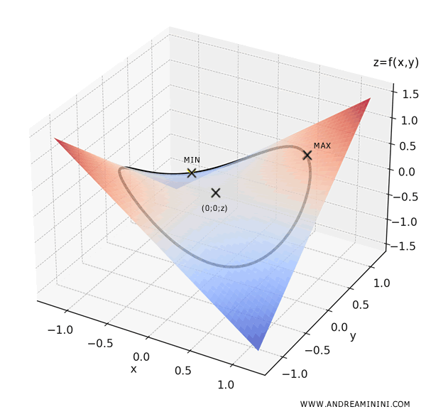
Thus, for this function, both the global maximum and minimum occur along the boundary of the domain, which is depicted by the black curve in the graph.

And what about the point \((0,0)\)? It turns out to be a saddle point - it is neither a maximum nor a minimum.

Example 3

Consider the function defined over the domain \( A = [0,1] \times [0,2] \).

\[ f(x,y) = 2x + 3y \]

The set \( A \) is closed and bounded, and therefore compact. The function \( f \) is continuous, as it is a polynomial in two variables.

By the Weierstrass theorem, \( f \) attains both an absolute maximum and an absolute minimum on \( A \).

In this case, determining the extrema is straightforward with a bit of intuitive reasoning.

Since \( f(x,y) \) is linear, it increases as either \( x \) or \( y \) increases.

Thus, the absolute minimum occurs when \( x \) and \( y \) take their smallest values in the domain, namely \( x = 0 \) and \( y = 0 \).

\[ f(0,0) = 2 \cdot 0 + 3 \cdot 0 = 0 \]

Conversely, the absolute maximum occurs when \( x \) and \( y \) reach their largest values allowed by the domain, that is, \( x = 1 \) and \( y = 2 \).

\[ f(1,2) = 2 \cdot 1 + 3 \cdot 2 = 2 + 6 = 8 \]

This example illustrates that when dealing with a simple function, such as a first-degree polynomial, it is possible to identify absolute extrema without resorting to derivative calculations - simply by analyzing the function’s behavior across the domain.

Level Curve Method

The level curve method is a graphical approach used to locate the maximum or minimum of a function \( f(x, y) \) over a set \( A \) (the function’s domain).

It’s an intuitive, visual technique, particularly effective for simple functions and polygonal domains.

How It Works

Here’s the step-by-step process:

1. Plot the set \( A \) in the \( (x,y) \) plane.
2. Draw the level curves of \( f(x, y) \), which are the curves along which the function remains constant:  \[ f(x, y) = \lambda \]
3. To find the maximum, identify the highest level curve (i.e., the one with the largest \( \lambda \)) that intersects or just touches \( A \). Similarly, the minimum corresponds to the lowest level curve that still meets \( A \).

Example

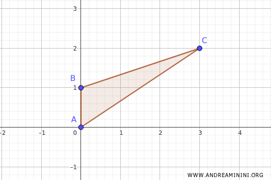
Let’s take \( f(x, y) = 2x - y \) with \( A \) being the triangle with vertices at \( (0,0) \), \( (0,1) \), and \( (3,2) \).

First, sketch the domain \( A \) in the plane, which in this case forms a triangle.

To determine the maximum and minimum of \( f(x, y) \) over \( A \), we construct the level curves of the function:

\[ f(x, y) = \lambda \]

\[ 2x - y = \lambda \]

\[ y = 2x - \lambda \]

Here, the level curves are parallel straight lines sloping downward with a slope of 2. As \( \lambda \) increases, the lines shift to the right.

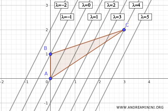
The highest level curve that still touches \( A \) passes through the point \( (3,2) \).

At this point, the function achieves its maximum value over \( A \):

\[ f(3, 2) = 2x - y = 2 \cdot 3 - 2 = 6 - 2 = 4 \]

To find the minimum, we follow the same logic, identifying the lowest level curve that still intersects the domain.

The lowest level curve touches \( A \) at the point \( (0,1) \).

At this point, the function attains its minimum value over \( A \):

\[ f(0, 1) = 2x - y = 2 \cdot 0 - 1 = -1 \]

Thus, by simply analyzing the level curves and the domain, we can determine both the maximum and minimum values of the function.

Parameterization Method

The parameterization method is a technique used to analyze a function and determine its absolute extrema over a bounded domain, particularly along its boundary.

It’s especially effective when examining a function \( f(x, y) \) defined on a closed and bounded region.

How the method works

The idea is to describe the boundary of the domain using parameterizations - transformations that express each portion of the boundary in terms of a single parameter \( t \).

1. Divide the boundary into simple segments (e.g., straight lines or curves).
2. Parameterize each segment with a function \( \gamma(t) = (x(t), y(t)) \) that traces it out.
3. Substitute into the original function to obtain \( f(x(t), y(t)) \), now a function of one variable.
4. Find the maximum and minimum values over each segment.
5. Repeat this process for all boundary segments.
6. Compare all resulting values to identify the global maximum and minimum over the domain.

This approach reduces a two-variable optimization problem to a collection of one-variable problems.

It is particularly useful for domains bounded by curves or straight edges, such as rectangles, circles, and polygons.

For instance, if one side of the boundary is the segment from \((x,y)= (2,1) \) to \( (x,y)=(5,1) \), a suitable parameterization is:  \[  x(t) = t,\quad y(t) = 1,\quad \text{with } t \in [2,5] \] The function \( f(x,y) \) is then rewritten as a function of a single variable: \[ f(x(t), y(t)) = f(t, 1) \]

Example

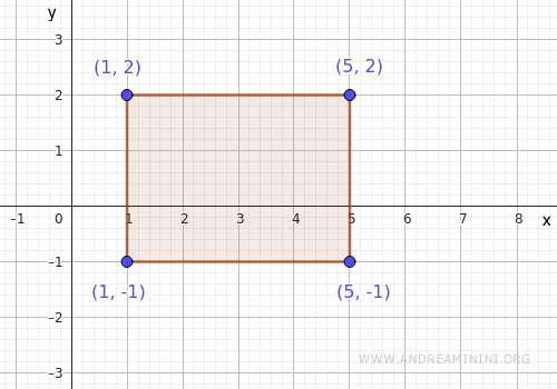
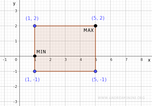
Consider the function

$$ f(x,y) = x^2 + y^2 $$

on the rectangular domain

$$ A = [1,5] \times [-1,2] $$

We aim to identify the points where the function reaches its minimum and maximum values over this domain.

We analyze three aspects: interior stationary points, interior singular points, and boundary behavior.

1] Interior stationary points

First, compute the gradient of the function:

\[ \nabla f(x,y) = (2x, 2y) \]

Then solve for where the gradient is zero:

$$ \begin{cases} 2x=0 \\ \\ 2y = 0 \end{cases} $$

This occurs at the point \( (0,0) \):

\[ \nabla f(x,y) = (0,0) \Rightarrow x = 0,\ y = 0 \]

However, \( (0,0) \) lies outside the domain \( [1,5] \times [-1,2] \), so there are no critical points in the interior.

2] Interior singular points

Next, check whether the function fails to be differentiable at any interior point (i.e., where partial derivatives don't exist).

In this case, the function is differentiable everywhere in the domain, so there are no interior singularities.

3] Boundary analysis

To study the function on the boundary, we apply the parameterization method.

The boundary of the rectangle consists of four sides. We examine each one in turn.

• Top side
  This is the horizontal segment from \( (1,2) \) to \( (5,2) \). We parameterize it as \( \gamma(t) = (t, 2) \), with \( t \in [1,5] \).
  
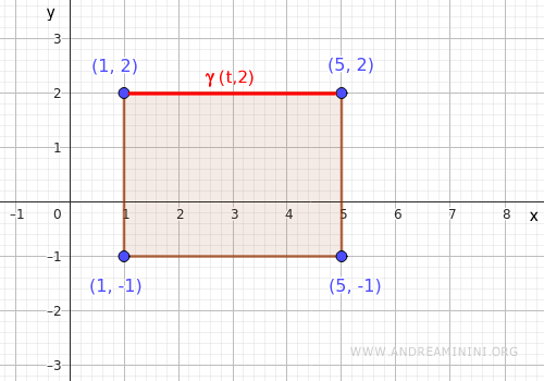
  Substituting into the function yields: $$ f(t,2) = t^2 + 4 $$ We then find the extrema over the interval \( t \in [1,5] \)
  • Minimum at \( t=1 \): \( f(1,2) = 1 + 4 = 5 \)
  • Maximum at \( t=5 \): \( f(5,2) = 25 + 4 = 29 \)
• Bottom side
  This horizontal segment runs from \( (1,-1) \) to \( (5,-1) \), parameterized as \( \gamma(t) = (t, -1) \), with \( t \in [1,5] \).
  
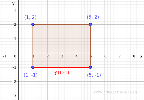
  Substituting into the function gives: $$ f(t,-1) = t^2 + 1 $$ We evaluate this on the interval \( t \in [1,5] \)
  • Minimum: \( f(1,-1) = 1 + 1 = 2 \) 
  • Maximum: \( f(5,-1) = 25 + 1 = 26 \)
• Right side
  This vertical segment goes from \( (5,-1) \) to \( (5,2) \), and is parameterized as \( \gamma(t) = (5, t) \), with \( t \in [-1,2] \).
  
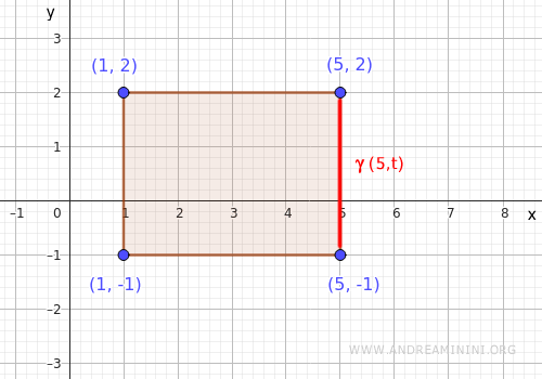
  Substituting into the function gives: $$ f(5,t) = 25 + t^2 $$ We analyze this on \( t \in [-1,2] \)
  • Minimum at \( t=0 \): \( f(5,0) = 25 + 0 = 25 \) 
  • Maximum at \( t=2 \): \( f(5,2) = 25 + 4 = 29 \)
• Left side
  This segment runs from \( (1,-1) \) to \( (1,2) \), and we parameterize it as \( \gamma(t) = (1, t) \), with \( t \in [-1,2] \).
  
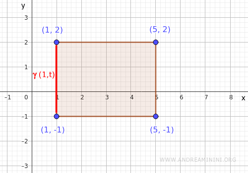
  Substituting into the function yields: $$ f(1,t) = 1 + t^2 $$ Then analyze this over \( t \in [-1,2] \)
  • Minimum: \( f(1,0) = 1 + 0 = 1 \)
  • Maximum: \( f(1,2) = 1 + 4 = 5 \)

Summarizing the results, we obtain the following candidate points on the boundary for global extrema:

\[
\begin{array}{|c|c|}
\hline
\textbf{Point} & \textbf{f(x,y)} & \textbf{Classification} \\
\hline
(1,2) &  5  &\\
(5,2) &  29 & maximum \\
(5,0) & 25 & \\
(5,-1) & 26 & \\
(1,-1) &  2 & \\
(1,0) & 1 & minimum \\
\hline
\end{array}
\]

Thus, the function \( x^2+y^2 \) attains its absolute minimum at \( (1,0) \) and its absolute maximum at \( (5,2) \). The other points can be discarded.

Method of Lagrange Multipliers

The method of Lagrange multipliers is a powerful tool for identifying local maxima and minima of a function subject to a constraint.

It's particularly effective when optimizing a function $f(x, y)$ under a constraint of the form $g(x, y) = 0$.

The goal is to find the points $(x, y)$ that either maximize or minimize $f(x, y)$, while satisfying the constraint $g(x, y) = 0$.

The core idea is that if $f(x, y)$ has an extremum under the constraint, then at that point the gradients of $f$ and $g$ must be parallel:

$$ \nabla f(x, y) = \lambda \nabla g(x, y) $$

Where:

• $\nabla f = \left( \frac{\partial f}{\partial x}, \frac{\partial f}{\partial y} \right)$ is the gradient of $f$
• $\nabla g = \left( \frac{\partial g}{\partial x}, \frac{\partial g}{\partial y} \right)$ is the gradient of the constraint $g$
• $\lambda$ is the Lagrange multiplier

How the method works

Here’s the procedure step by step:

1. Set up the following system: $$
   \begin{cases}
   \frac{\partial f}{\partial x} = \lambda \frac{\partial g}{\partial x} \\
   \frac{\partial f}{\partial y} = \lambda \frac{\partial g}{\partial y} \\
   g(x, y) = 0
   \end{cases}
   $$
2. Solve the resulting system of three equations in the unknowns $x$, $y$, and $\lambda$
3. Identify the critical points $(x, y)$
4. Evaluate $f(x, y)$ at each critical point to determine which values correspond to a maximum or a minimum

Note. This method yields candidate points where extrema may occur, but it doesn’t automatically distinguish between maxima and minima. Each point must be tested to determine its nature.

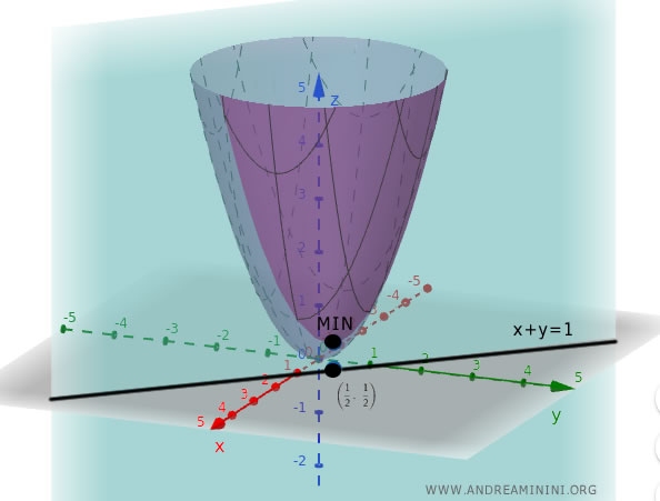
Worked Example

Consider the function:

$$ f(x, y) = x^2 + y^2 $$

subject to the constraint:

$$ x + y = 1 $$

First, rewrite the constraint as an equation of the form $g(x, y) = 0$:

$$ g(x, y) = x + y - 1 = 0 $$

Next, compute the gradients:

$$ \nabla f = (2x, 2y) $$

$$ \nabla g = (1, 1) $$

Now construct the system of equations using the method of Lagrange multipliers:

$$ \begin{cases}
2x = \lambda \cdot 1 \\
2y = \lambda \cdot 1 \\
x + y = 1
\end{cases}
\Rightarrow
\begin{cases}
\lambda = 2x \\
\lambda = 2y \\
x + y = 1
\end{cases}
$$

Substituting $\lambda = 2x$ into the second equation gives $2x = 2y$, so $x = y$.

Substitute into the constraint:

$$ \begin{cases}
\lambda = 2x \\
x = y \\
x + x = 1
\end{cases} \Rightarrow
\begin{cases}
\lambda = 2x \\
x = y \\
2x = 1
\end{cases} \Rightarrow
\begin{cases}
\lambda = 2x \\
x = y \\
x = \frac{1}{2}
\end{cases} $$

Since $x = y$, it follows that $y = \frac{1}{2}$ as well:

$$ \begin{cases}
\lambda = 2x \\
y = \frac{1}{2} \\
x = \frac{1}{2}
\end{cases} $$

So the critical point to evaluate is $ \left( \frac{1}{2}, \frac{1}{2} \right) $

Evaluate the function at this point:

$$ f \left( \frac{1}{2}, \frac{1}{2} \right) = \left( \frac{1}{2} \right)^2 + \left( \frac{1}{2} \right)^2 = \frac{1}{2} $$

Since the function $f(x, y) = x^2 + y^2$ increases with distance from the origin and the constraint defines a straight line, this critical point corresponds to a minimum under the constraint $x + y = 1$.

Method of Stationary Points of the Constraint

The stationary point system of the constraint refers to the set of equations that identify the points where the gradient of the constraint function vanishes. Specifically: $$ \begin{cases} \Phi(x, y) = 0 \\ \frac{\partial \Phi}{\partial x}(x, y) = 0 \\ \frac{\partial \Phi}{\partial y}(x, y) = 0 \end{cases} $$ where $\Phi(x, y)$ denotes the constraint function.

These points are called stationary points of the constraint because at each of them, the constraint’s gradient is zero.

Geometrically, this means the constraint curve exhibits some form of singular behavior at those locations - such as a cusp, a corner, or a point where the curve fails to be smooth.

This method is especially useful when the gradient of the constraint vanishes, making the Lagrange multipliers method inapplicable.

Note: The Lagrange multiplier method assumes that the gradient of the constraint is non-zero. If the gradient vanishes, the regularity conditions fail, and the method cannot be applied.

That said, this approach does not guarantee solutions: the resulting system may be inconsistent or may have no real solutions at all.

And even when real solutions exist, they must be examined individually to determine whether they correspond to local maxima, minima, or neither.

In short, stationary points of the constraint are potential candidates for constrained extrema and must be analyzed on a case-by-case basis.

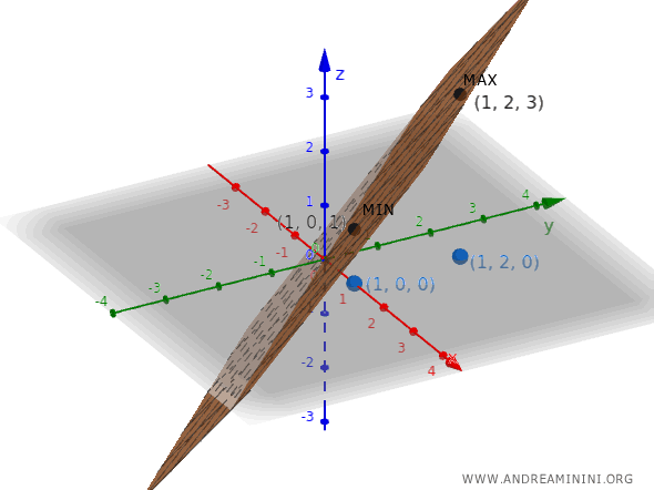
Example

Consider the function:

$$ f(x,y) = x + y $$

subject to the constraint:

$$ \Phi(x, y) = (x - 1)^2 + y^2(y - 2)^2 $$

We begin by computing the partial derivatives of the constraint:

$$ \frac{\partial \Phi}{\partial x} = 2(x - 1) $$

$$ \frac{\partial \Phi}{\partial y} = 2y(y - 2)^2 + 2y^2(y - 2) $$

We now solve the system:

$$
\begin{cases}
\Phi(x, y) = 0 \\
\frac{\partial \Phi}{\partial x}(x, y) = 0 \\
\frac{\partial \Phi}{\partial y}(x, y) = 0
\end{cases}
$$

That is:

$$ \begin{cases}
(x - 1)^2 + y^2(y - 2)^2 = 0 \\
2(x - 1) = 0 \\
2y(y - 2)^2 + 2y^2(y - 2) = 0
\end{cases} $$

The second equation immediately gives $x = 1$.

Substituting this into the first equation yields:

$$ (1 - 1)^2 + y^2(y - 2)^2 = 0 \quad \Rightarrow \quad y = 0 \quad \text{or} \quad y = 2 $$

Thus, the candidate points are:

$$ (1, 0) \quad \text{and} \quad (1, 2) $$

Evaluating $f$ at each point gives:

$$ f(1, 0) = 1 $$

$$ f(1, 2) = 3 $$

Therefore, $ (1, 0) $ is a local minimum ( $ f = 1 $ ), and $ (1, 2) $ is a local maximum ( $ f = 3 $ ) under the constraint.

It is important to observe that in this case, the constraint $ \Phi(x, y) = 0 $ reduces to exactly two isolated points: $ (1, 0) $ and $ (1, 2) $. Once this is recognized, the full analytical procedure becomes unnecessary, as the problem reduces to simply evaluating the objective function at these two candidates.

Note: In this example, the Lagrange multiplier method cannot be used because the gradient of the constraint vanishes at both points: $\nabla \Phi = 0$. Recall that the gradient of the constraint is: $$ \nabla \Phi(x, y) = \left( \frac{\partial \Phi}{\partial x}, \frac{\partial \Phi}{\partial y} \right) $$ We compute the components: $$ \frac{\partial \Phi}{\partial x} = 2(x - 1) $$ $$ \frac{\partial \Phi}{\partial y} = \frac{\partial}{\partial y} \left[ y^2(y - 2)^2 \right] $$ At the point $ (1, 0) $: $$ \frac{\partial \Phi}{\partial x} = 2(0) = 0 $$ $$ \frac{\partial \Phi}{\partial y} = 2 \cdot 0 \cdot 4 + 2 \cdot 0^2 \cdot (-2) = 0 $$ At the point $ (1, 2) $: $$ \frac{\partial \Phi}{\partial x} = 0 $$ $$ \frac{\partial \Phi}{\partial y} = 2 \cdot 2 \cdot 0 + 2 \cdot 4 \cdot 0 = 0 $$ So in both cases: $$ \nabla \Phi(1, 0) = (0, 0) \quad \text{and} \quad \nabla \Phi(1, 2) = (0, 0) $$ Hence, there is no value of $ \lambda $ that satisfies the Lagrange condition: $$ \nabla f = \lambda \nabla \Phi \quad \Rightarrow \quad \nabla f = \lambda (0, 0) = (0, 0) $$ This is not possible, so the method of Lagrange multipliers cannot be applied in this case.

Hessian Matrix

To identify local minima and maxima of a function of two variables, such as \( f(x, y) \), we can make use of the Hessian matrix.

The Hessian matrix is a square matrix consisting of all the second-order partial derivatives of the function:\[
H = \begin{pmatrix}
\frac{\partial^2 f}{\partial x^2} & \frac{\partial^2 f}{\partial x \partial y} \\
\frac{\partial^2 f}{\partial y \partial x} & \frac{\partial^2 f}{\partial y^2}
\end{pmatrix}
\]

The main diagonal contains the pure second partial derivatives, \( \frac{ \partial^2 f}{\partial x^2} \) and \( \frac{\partial^2 f}{\partial y^2 } \), where the same variable is differentiated twice.

The off-diagonal entries contain the mixed second partial derivatives, \( \frac{\partial^2 f}{\partial x \partial y} \) and \( \frac{\partial^2 f}{\partial y \partial x} \), involving differentiation first with respect to one variable and then the other.

Once the Hessian matrix is constructed, we substitute the coordinates of the critical point we wish to analyze into the matrix, replacing \( x \) and \( y \) with their respective values.

Note. If the Hessian is composed entirely of constants, it can be used directly without substitution to assess any critical point.

Next, we compute the determinant \( \Delta \) of the Hessian matrix:

• If \( \Delta > 0 \) and \( \frac{\partial^2 f}{\partial x^2} > 0 \), the point is a local minimum.
• If \( \Delta > 0 \) and \( \frac{\partial^2 f}{\partial x^2} < 0 \), the point is a local maximum.
• If \( \Delta < 0 \), the point is a saddle point - neither a minimum nor a maximum.
• If \( \Delta = 0 \), the Hessian test is inconclusive, and further analysis is required.

Example

In the previous exercise, we considered the function:

\[ f(x,y) = xy \]

over the domain:

\[ D = \{ (x,y) \, | \, x^2 + y^2 \leq 1 \} \]

where we identified a critical point at \( P(0,0) \).

To determine the nature of this critical point, we construct the Hessian matrix for the function:

\[
H = \begin{pmatrix}
\frac{\partial^2 f}{\partial x^2} & \frac{\partial^2 f}{\partial x \partial y} \\
\frac{\partial^2 f}{\partial y \partial x} & \frac{\partial^2 f}{\partial y^2}
\end{pmatrix}
\]

The first-order partial derivatives are:

• \( \frac{\partial f}{\partial x} = y \)
• \( \frac{\partial f}{\partial y} = x \)

The second-order partial derivatives, which we need for the Hessian, are:

• \(\frac{\partial^2 f}{\partial x^2} = 0\) (since \(y\) does not depend on \(x\))
• \(\frac{\partial^2 f}{\partial y^2} = 0\) (since \(x\) does not depend on \(y\))
• \(\frac{\partial^2 f}{\partial x \partial y} = 1\) (the derivative of \(y\) with respect to \(y\) is 1)
• \(\frac{\partial^2 f}{\partial y \partial x} = 1\) (the derivative of \(x\) with respect to \(x\) is 1)

Thus, the Hessian matrix is:

\[ H = \begin{pmatrix}
0 & 1 \\
1 & 0
\end{pmatrix}
\]

Since the matrix entries are constants, we can apply the Hessian test directly at \( P(0,0) \) without any substitution.

We now compute the determinant of the Hessian:

\[ \Delta = (0)(0) - (1)(1) = -1 \]

The determinant is negative, \(\Delta < 0\), indicating that \( P(0,0) \) is a saddle point - neither a local maximum nor a local minimum.

This conclusion is consistent with our earlier findings using direct methods.

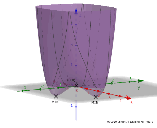
Example 2

Let’s examine the function:

\[ f(x,y) = x^4 - 2xy + y^4 \]

defined over the domain:

\[ D = \{ (x,y) \mid x^2 + y^2 \leq 4 \} \]

This corresponds to a circle of radius 2 centered at the origin \((0,0)\).

First, we compute the first-order partial derivatives:

• \(\frac{\partial f}{\partial x} = 4x^3 - 2y\)
• \(\frac{\partial f}{\partial y} = 4y^3 - 2x\)

Setting them equal to zero, we obtain the system:

\[ \begin{cases} 4x^3 - 2y = 0 \\ \\ 4y^3 - 2x = 0 \end{cases} \]

Solving the system:

\[ \begin{cases} y = 2x^3 \\ \\ 4(2x^3)^3 - 2x = 0 \end{cases} \]

\[ \begin{cases} y = 2x^3 \\ \\ 32x^9 - 2x = 0 \end{cases} \]

\[ \begin{cases} y = 2x^3 \\ \\ 2x(16x^8 - 1) = 0 \end{cases} \]

Thus, the solutions are \( x = 0 \) or \( 16x^8 = 1 \), which yields:

\[ x = \pm \frac{1}{\sqrt[8]{16}} = \pm \frac{1}{\sqrt[8]{2^4}} = \pm \frac{1}{\sqrt{2}} \approx \pm 0.707 \]

Substituting these values into the first equation \(y = 2x^3\) gives:

• If \(x = 0\), then \(y = 0\).
• If \(x = \frac{1}{\sqrt{2}}\), then \[ y = 2\left(\frac{1}{\sqrt{2}}\right)^3 = 2\left(\frac{1}{2\sqrt{2}}\right) = \frac{1}{\sqrt{2}}. \]
• If \(x = -\frac{1}{\sqrt{2}}\), then \[ y = 2\left(-\frac{1}{\sqrt{2}}\right)^3 = 2\left(-\frac{1}{2\sqrt{2}}\right) = -\frac{1}{\sqrt{2}}. \]

Thus, the critical points are:

• \((0,0)\)
• \(\left(\frac{1}{\sqrt{2}}, \frac{1}{\sqrt{2}}\right)\)
• \(\left(-\frac{1}{\sqrt{2}}, -\frac{1}{\sqrt{2}}\right)\)

All of these points lie inside the circle of radius 2, as they satisfy \((x^2 + y^2) \leq 4\).

We now proceed to construct the Hessian matrix.

The second-order partial derivatives are:

• \(\frac{\partial^2 f}{\partial x^2} = 12x^2\)
• \(\frac{\partial^2 f}{\partial y^2} = 12y^2\)
• \(\frac{\partial^2 f}{\partial x \partial y} = \frac{\partial^2 f}{\partial y \partial x} = -2\)

Thus, the Hessian matrix takes the form:

\[
H = \begin{pmatrix}
12x^2 & -2 \\
-2 & 12y^2
\end{pmatrix}
\]

Let’s evaluate the Hessian at each critical point.

1] At \((0,0)\):

Substituting \(x = 0\) and \(y = 0\):

\[
H(0,0) = \begin{pmatrix}
0 & -2 \\
-2 & 0
\end{pmatrix}
\]

Computing the determinant:

\[ \Delta = (0)(0) - (-2)(-2) = -4 \]

Since the determinant is negative \((\Delta < 0)\), \((0,0)\) is a saddle point.

2] At \(\left(\frac{1}{\sqrt{2}}, \frac{1}{\sqrt{2}}\right)\):

Substituting \(x = \frac{1}{\sqrt{2}}\) and \(y = \frac{1}{\sqrt{2}}\):

\[
H\left(\frac{1}{\sqrt{2}}, \frac{1}{\sqrt{2}}\right) = \begin{pmatrix}
12\left(\frac{1}{2}\right) & -2 \\
-2 & 12\left(\frac{1}{2}\right)
\end{pmatrix} = \begin{pmatrix}
6 & -2 \\
-2 & 6
\end{pmatrix}
\]

Computing the determinant:

\[ \Delta = (6)(6) - (-2)(-2) = 36 - 4 = 32 \]

Since \(\Delta > 0\) and \(\frac{\partial^2 f}{\partial x^2} = 6 > 0\), the point is a local minimum.

3] At \(\left(-\frac{1}{\sqrt{2}}, -\frac{1}{\sqrt{2}}\right)\):

By symmetry, the calculation is identical:

\[
H\left(-\frac{1}{\sqrt{2}}, -\frac{1}{\sqrt{2}}\right) = \begin{pmatrix}
6 & -2 \\
-2 & 6
\end{pmatrix}
\]

The determinant remains:

\[ \Delta = (6)(6) - (-2)(-2) = 32 \]

Thus, this point is also a local minimum.

And so forth.