Absolute and Relative Frequency: Definition and Examples
What Is Frequency?
In statistics, frequency describes how often a particular value, category, or event occurs in a data set.
Whenever statisticians collect data, one of the first questions they ask is: How often does each value occur? The answer is provided by frequency.
Frequency is one of the most important tools for organizing and understanding data. It allows us to summarize large amounts of information, identify patterns, compare groups, and draw meaningful conclusions from observations.
There are two main types of frequency: absolute frequency and relative frequency.
- Absolute Frequency
Absolute frequency is the number of times a particular value or category appears in a data set.Example: Suppose a group consists of 50 people, 30 of whom are female. The absolute frequency of females is 30.
- Relative Frequency
Relative frequency indicates the proportion of observations that belong to a particular category or have a particular value. It is calculated by dividing the absolute frequency (F) by the total number of observations (T): $$ f = \frac{F}{T} $$ Relative frequency can be expressed either as a decimal or as a percentage.Example: In a group of 50 people, if 30 are female, the relative frequency of females is: $$ f = \frac{30}{50} = 0.6 $$ This means that 60% of the group is female.
The sum of all relative frequencies in a data set is always equal to 1, or 100% when expressed as percentages.
A Practical Example
Let's see how absolute and relative frequencies are used in practice.
The following frequency table shows the gender distribution of students in a class:
| Category | Absolute Frequency | Relative Frequency | % |
|---|---|---|---|
| Male | 8 | 0.4 | 40% |
| Female | 12 | 0.6 | 60% |
| Total | 20 | 1 | 100% |
The statistical variable being studied is gender, which has two categories: male (M) and female (F).
The class contains 20 students, which is the total number of observations.
Note: The complete set of individuals under study is called the population, while each individual observation is known as a statistical unit.
There are 8 male students and 12 female students. These values represent the absolute frequencies of the two categories.
To find the relative frequencies, divide each absolute frequency by the total number of observations:
$$ \frac{8}{20} = 0.4 $$
$$ \frac{12}{20} = 0.6 $$
These results tell us that 40% of the students are male and 60% are female.
Note: To convert a relative frequency into a percentage, simply multiply it by 100.
$$ 0.4 \times 100 = 40\% $$
$$ 0.6 \times 100 = 60\% $$
As expected, the relative frequencies add up to 1:
$$ 0.4 + 0.6 = 1 $$
or, in percentage form:
$$ 40\% + 60\% = 100\% $$
The table therefore provides a complete summary of the distribution of students by gender.
| Category | Absolute Frequency | Relative Frequency | % |
|---|---|---|---|
| Male | 8 | 0.4 | 40% |
| Female | 12 | 0.6 | 60% |
| Total | 20 | 1 | 100% |
This type of table is called a frequency table.
The collection of categories and their corresponding frequencies forms the frequency distribution:
$$ (M,8) \\ (F,12) $$
The Relationship Between Absolute and Relative Frequency
Absolute frequency and relative frequency describe the same information from two different perspectives.
Absolute frequency tells us how many observations belong to a category, while relative frequency tells us what proportion of the total they represent.
The relationship between them is straightforward.
To calculate the relative frequency:
$$ f = \frac{F}{T} $$
To calculate the absolute frequency:
$$ F = f \cdot T $$
For example, suppose the relative frequency of male students is 0.4 and the class contains 20 students. The corresponding absolute frequency is:
$$ F = 0.4 \cdot 20 = 8 $$
If the relative frequency is expressed as a percentage, first convert it to decimal form:
$$ 40\% = \frac{40}{100} = 0.4 $$
Then apply the formula:
$$ F = 0.4 \cdot 20 = 8 $$
Frequency Classes
When a statistical variable can take many different values, it is often useful to group those values into frequency classes. Each class represents a range of values rather than a single value.
Consider the heights of 20 students.
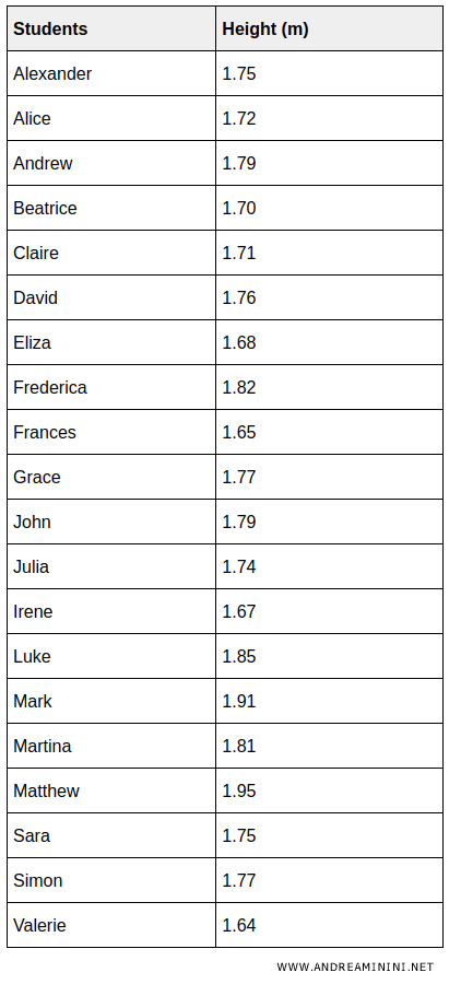
Because every student may have a slightly different height, listing each value separately can make the data difficult to interpret. In these situations, grouping observations into classes provides a clearer overview of the distribution.
For example, we can divide the height measurements into four frequency classes and count how many students fall within each interval.
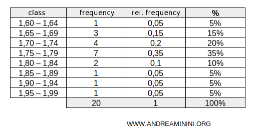
Instead of focusing on individual values, we can now see how the observations are distributed across broader ranges.
This produces a more compact summary of the data and often makes overall trends easier to identify.
Note: Grouping observations into classes inevitably reduces some detail, but it usually provides a clearer picture of the overall distribution.
When working with grouped data, it is common to calculate a representative value for each class.
This value is called the class midpoint and is obtained by taking the arithmetic mean of the lower and upper class limits.
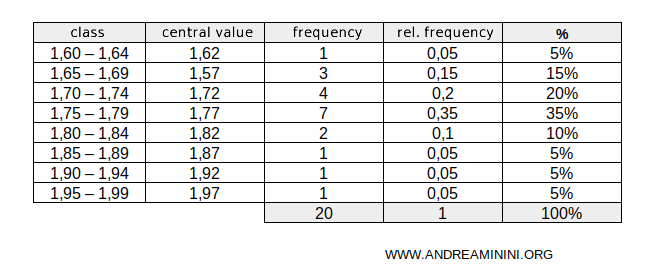
Example: Consider the class interval 1.60 - 1.64. The lower class limit is 1.60 and the upper class limit is 1.64. The class midpoint is:
$$ \frac{1.60 + 1.64}{2} = 1.62 $$
The class midpoint serves as a representative value for all observations within the interval and is particularly useful when calculating statistical measures from grouped data.


