Analytic Geometry

Analytic geometry, also known as Cartesian geometry, is a branch of mathematics that combines algebra and geometry to describe, analyze, and solve geometric problems.

Its central idea is simple yet powerful: geometric objects can be represented by equations, and geometric relationships can be studied using algebraic techniques.

By introducing coordinates, analytic geometry makes it possible to translate shapes, curves, and spatial relationships into mathematical expressions that can be manipulated and solved systematically.

How does it differ from Euclidean geometry?

Traditional Euclidean geometry is based on axioms, logical deductions, and geometric constructions, such as those derived from Euclid’s postulates.

Analytic geometry takes a different approach. Instead of relying primarily on geometric constructions, it uses coordinates such as \((x,y)\) and \((x,y,z)\) to represent geometric objects and studies them through algebraic equations.

This approach allows mathematicians to analyze points, lines, curves, planes, and surfaces using a common mathematical language.

The two fundamental pillars of analytic geometry are:

• Equations
  Every geometric object can be represented by an equation. For example, a straight line in the plane can be described by the linear equation \(ax+by+c=0\), while a circle centered at the origin is represented by the equation \(x^2+y^2=r^2\), where \(r\) is the radius.
  
  More advanced equations can describe conic sections such as parabolas, ellipses, and hyperbolas, as well as surfaces in three-dimensional space.
• Coordinate Systems
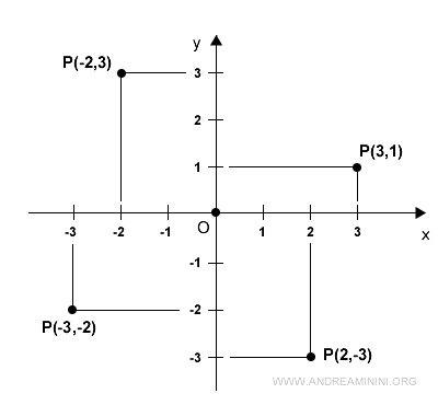
  The most commonly used coordinate system is the Cartesian coordinate system, known in two dimensions as the Cartesian plane.
  
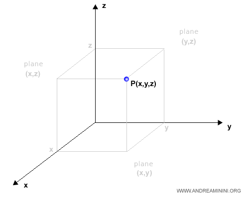
  It consists of two or three perpendicular axes used to locate points in a plane or in space. Each point is identified by a set of coordinates, written as \((x,y)\) in two dimensions or \((x,y,z)\) in three dimensions.
  
  These coordinates indicate the point’s position relative to the coordinate axes.
  
  In three-dimensional Cartesian space, every point is specified by three coordinates, \((x,y,z)\), corresponding to its position along the \(x\)-, \(y\)-, and \(z\)-axes.
  

One of the main goals of analytic geometry is to determine where curves or surfaces intersect. In practice, this means solving systems of equations whose solutions correspond to the points of intersection.

Analytic geometry also provides practical methods for calculating distances, angles, slopes, tangents, areas, and many other geometric quantities directly from coordinates and equations.

The Origins of Analytic Geometry. Analytic geometry emerged during the seventeenth century through the groundbreaking work of René Descartes and Pierre de Fermat. By bringing algebra and geometry together within a single framework, they transformed the way mathematicians approached geometric problems.

Because of Descartes' influential role, analytic geometry is often called Cartesian geometry. The ideas introduced during this period later became essential for the development of differential and integral calculus, classical mechanics, and many areas of modern mathematics and physics.

A Practical Example

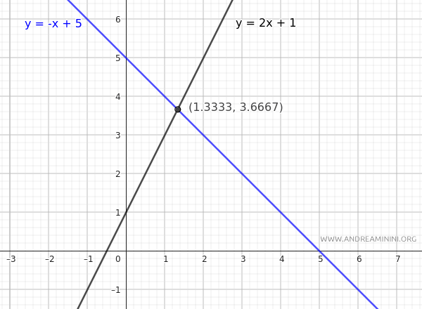
One of the most common applications of analytic geometry is finding the point where two lines intersect.

Consider the following lines in the Cartesian plane:

$$ L_1: y = 2x + 1 $$

$$ L_2: y = -x + 5 $$

The point of intersection is the point whose coordinates satisfy both equations at the same time.

To find it, we solve the following system of equations:

$$ \begin{cases} y = 2x + 1 \\ y = -x + 5 \end{cases} $$

Since both expressions are equal to \(y\), we can set them equal to each other:

$$ \begin{cases} -x + 5 = 2x + 1 \\ y = -x + 5 \end{cases} $$

$$ \begin{cases} -x - 2x = -5 + 1 \\ y = -x + 5 \end{cases} $$

$$ \begin{cases} -3x = -4 \\ y = -x + 5 \end{cases} $$

$$ \begin{cases} x = \frac{4}{3} \\ y = -x + 5 \end{cases} $$

Now substitute \(x=\frac{4}{3}\) into one of the original equations:

$$ \begin{cases} x = \frac{4}{3} \\ y = -\left(\frac{4}{3}\right) + 5 \end{cases} $$

$$ \begin{cases} x = \frac{4}{3} \\ y = \frac{-4 + 15}{3} \end{cases} $$

$$ \begin{cases} x = \frac{4}{3} \\ y = \frac{11}{3} \end{cases} $$

In decimal form, this becomes:

$$ \begin{cases} x = 1.3333 \\ y = 3.6667 \end{cases} $$

Therefore, the two lines intersect at the point

$$ \left(\frac{4}{3},\frac{11}{3}\right) $$

or approximately

$$ (1.3333,\;3.6667) $$

This example highlights one of the key strengths of analytic geometry: geometric problems can be transformed into algebraic calculations and solved with precision.

The same methods can be applied to many other problems, from finding distances and angles to studying curves, surfaces, and geometric transformations.