Mean Value Theorem
What the Mean Value Theorem Says
Let \( f(x) \) be a function that is continuous on the closed interval \( [a,b] \) and differentiable on the open interval \( (a,b) \). Then there exists at least one point \(x_0 \in (a,b) \) where the derivative of the function is equal to the slope of the secant line connecting the points \( (a,f(a)) \) and \( (b,f(b)) \):$$ f'(x_0)=\frac{f(b)-f(a)}{b-a} $$
The Mean Value Theorem is one of the most important results in differential calculus. It's also called Lagrange's Mean Value Theorem.
It establishes a direct connection between the average rate of change of a function over an interval and its instantaneous rate of change at a specific point within that interval.
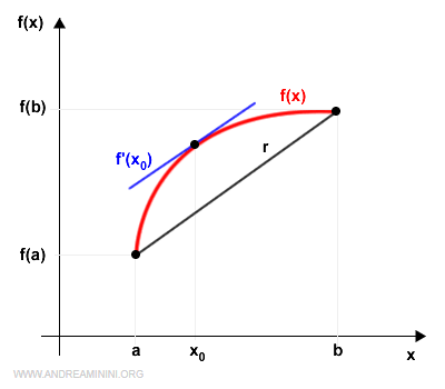
Geometrically, the theorem guarantees that there is at least one point in the interval \( (a,b) \) where the tangent line to the graph of the function is parallel to the secant line joining the endpoints \( (a,f(a)) \) and \( (b,f(b)) \).
In other words, at some point inside the interval, the function's instantaneous rate of change is exactly equal to its average rate of change over the entire interval.
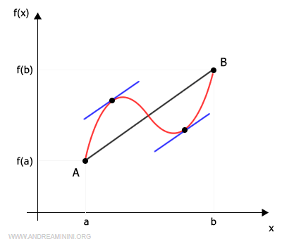
The theorem guarantees the existence of at least one such point, although there may be several points that satisfy this condition.
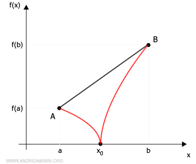
Note. Continuity alone is not sufficient to apply the Mean Value Theorem. The function must also be differentiable throughout the open interval \( (a,b) \). For example, the function shown below has equal endpoint values \( f(a)=f(b) \) and is continuous on \( [a,b] \), but it is not differentiable at the point \( x_0 \in (a,b) \). As a result, there is no point where the tangent line is parallel to the line \( AB \).
A Worked Example
Let's apply the Mean Value Theorem to the function
$$ f(x)=x^2 $$
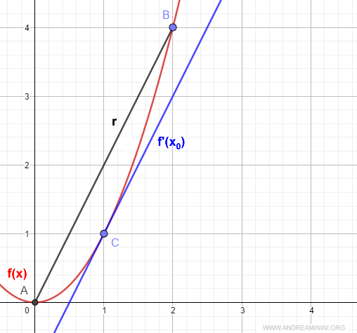
This function is continuous on the interval [0,2] and differentiable on (0,2), so the theorem applies.
According to the theorem, we need to find the point \( x_0 \) such that
$$ f'(x_0) = \frac{f(b)-f(a)}{b-a} $$
The derivative of \( f(x)=x^2 \) is
$$ f'(x)=2x $$
Substituting this into the formula gives
$$ 2x_0 = \frac{f(b)-f(a)}{b-a} $$
Since the endpoints of the interval are \( a=0 \) and \( b=2 \), we obtain
$$ 2x_0 = \frac{f(2)-f(0)}{2-0} $$
$$ 2x_0 = \frac{4-0}{2-0} $$
$$ 2x_0 = 2 $$
Solving for \( x_0 \), we get
$$ x_0 = \frac{2}{2} = 1 $$
Therefore, the point required by the Mean Value Theorem is
$$ x_0 = 1 $$
At \( x_0=1 \), the derivative of the function is equal to the slope of the secant line joining the endpoints of the interval. In this case, the instantaneous rate of change matches the average rate of change exactly as predicted by the theorem.
Proof and Explanation
Let’s take a function f(x) that’s continuous on [a,b] and differentiable on (a,b).
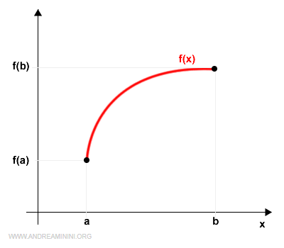
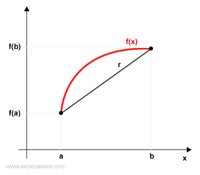
The equation of the line connecting the endpoints a and b is:
$$ r: f(a) + \frac{f(b)-f(a)}{b-a} \cdot (x - a) $$
Here’s how it appears on a Cartesian plane:
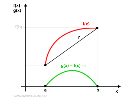
Now, define a new function g(x) to represent the difference between f(x) and the line r:
$$ g(x) = f(x) - r $$
$$ g(x) = f(x) - \left[ f(a) + \frac{f(b)-f(a)}{b-a} \cdot (x - a) \right] $$
This difference, f(x) - r, is zero at both endpoints a and b.
So, g(x) is also zero at those points.
Verification. At x = a, the function g(x) equals zero: $$ g(x) = f(x) - \left[ f(a) + \frac{f(b)-f(a)}{b-a} \cdot (x - a) \right] $$ $$ g(a) = f(a) - \left[ f(a) + \frac{f(b)-f(a)}{b-a} \cdot (a - a) \right] $$ $$ g(a) = f(a) - \left[ f(a) + \frac{f(b)-f(a)}{b-a} \cdot 0 \right] $$ $$ g(a) = f(a) - f(a) $$ $$ g(a) = 0 $$
At x = b, the function g(x) is also zero: $$ g(x) = f(x) - \left[ f(a) + \frac{f(b)-f(a)}{b-a} \cdot (x - a) \right] $$ $$ g(b) = f(b) - \left[ f(a) + \frac{f(b)-f(a)}{b-a} \cdot (b - a) \right] $$ $$ g(b) = f(b) - \left[ f(a) + f(b) - f(a) \right] $$ $$ g(b) = f(b) - f(b) $$ $$ g(b) = 0 $$
Since g(x) is zero at both endpoints,
$$ g(a) = g(b) = 0 $$
by the Rolle’s Theorem, there must be at least one point x ∈ (a,b) where the derivative is zero:
$$ g'(x_0)=0 $$
Let’s differentiate g(x) on the interval (a,b):
$$ D[g(x)] = D\left[ f(x) - \left( f(a) + \frac{f(b)-f(a)}{b-a} \cdot (x - a) \right) \right] $$
$$ g'(x) = D[f(x)] - D\left[ f(a) + \frac{f(b)-f(a)}{b-a} \cdot (x - a) \right] $$
$$ g'(x) = f'(x) - \frac{f(b)-f(a)}{b-a} $$
Since g'(x) = 0 at x0, we have:
$$ 0 = f'(x) - \frac{f(b)-f(a)}{b-a} $$
From this, it follows that the first derivative equals the slope of the line connecting a and b:
$$ f'(x) = \frac{f(b)-f(a)}{b-a} $$
Geometrically, the tangent line at x0 - that is, the derivative f'(x0) - shares the same slope as the secant line r.
We have thus proven Lagrange’s Theorem.
Geometric Interpretation. Let's take a closer look at the graph used in the previous proof.
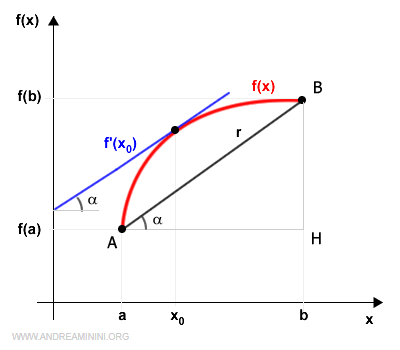
The Mean Value Theorem tells us that there is at least one point \( x_0 \) where the tangent line to the curve is parallel to the secant line \( AB \). Since parallel lines have the same slope, we can write
$$ \tan \alpha = f'(x_0) $$
Now consider the right triangle \( ABH \). From elementary trigonometry, the tangent of an angle is equal to the ratio of the opposite side to the adjacent side. Therefore,
$$ \overline{HB} = \overline{AH} \cdot \tan \alpha $$
Solving for \( \tan \alpha \), we obtain
$$ \tan \alpha = \frac{\overline{HB}}{\overline{AH}} $$
Since \( \overline{HB}=f(b)-f(a) \) and \( \overline{AH}=b-a \), this becomes
$$ \tan \alpha = \frac{f(b)-f(a)}{b-a} $$
Finally, substituting \( \tan \alpha = f'(x_0) \), we get
$$ f'(x_0) = \frac{f(b)-f(a)}{b-a} $$
This is exactly the statement of the Mean Value Theorem.
An Alternative Proof
There is another elegant way to prove the Mean Value Theorem using Rolle's Theorem.
Let \( f(x) \) be a function that is continuous on \( [a,b] \) and differentiable on \( (a,b) \).
Define the auxiliary function
\[ F(x)=f(x)-kx \]
where \( k \) is a real constant.
Because \( f(x) \) is continuous on \( [a,b] \) and differentiable on \( (a,b) \), the function \( F(x) \) inherits the same properties. Subtracting a linear function does not affect continuity or differentiability.
We now choose the constant \( k \) so that the auxiliary function takes the same value at both endpoints:
\[ F(a)=F(b) \]
Once this condition is satisfied, Rolle's Theorem can be applied.
Since \( F(a)=f(a)-ka \) and \( F(b)=f(b)-kb \), we have
\[ f(a)-ka=f(b)-kb \]
Solving this equation for \( k \),
\[ f(a)-f(b)=ka-kb \]
\[ f(a)-f(b)=k(a-b) \]
\[ k=\frac{f(a)-f(b)}{a-b} \]
Multiplying both the numerator and denominator by \( -1 \), we obtain
\[ k=\frac{f(b)-f(a)}{b-a} \]
Substituting this value into the definition of \( F(x) \), we get
\[ F(x)=f(x)-\frac{f(b)-f(a)}{b-a}x \]
The function \( F(x) \) now satisfies all the hypotheses of Rolle's Theorem. It is continuous on \([a,b]\), differentiable on \((a,b)\), and satisfies \( F(a)=F(b) \).
Therefore, Rolle's Theorem guarantees the existence of at least one point \( c \in (a,b) \) such that
\[ F'(c)=0 \]
Next, compute the derivative of \( F(x) \):
\[ F'(x)=f'(x)-\frac{f(b)-f(a)}{b-a} \]
Evaluating the derivative at \( c \), we obtain
\[ F'(c)=f'(c)-\frac{f(b)-f(a)}{b-a} \]
Since \( F'(c)=0 \), it follows that
\[ f'(c)-\frac{f(b)-f(a)}{b-a}=0 \]
Adding the second term to both sides gives
\[ f'(c)=\frac{f(b)-f(a)}{b-a} \]
This is precisely the conclusion of the Mean Value Theorem. Therefore, the theorem has been proved.
Q.E.D.
Notes
The following corollary is one of the most important consequences of Lagrange’s Mean Value Theorem. It provides a simple criterion for determining whether a function is constant on an interval.
- Corollary: A Function with Zero Derivative Is Constant
If a function f(x) is continuous on the interval [a,b], differentiable on the interval (a,b), and satisfies $ f'(x)=0 $ for every $ x \in (a,b) $, then the function must be constant throughout the interval [a,b].
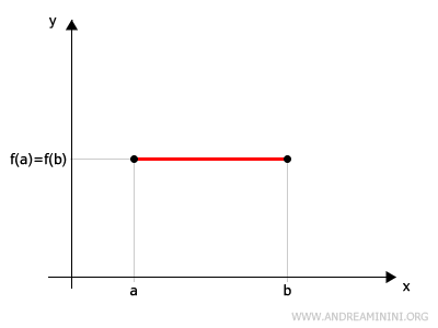
Proof. Let \( x_1,x_2 \in [a,b] \) with \(x_1<x_2 \). Since \( f \) is continuous on \([a,b] \) and differentiable on \((a,b) \), it is also continuous on \([x_1,x_2] \) and differentiable on \((x_1,x_2) \). By Lagrange’s Mean Value Theorem, there exists at least one point \(c \in (x_1,x_2) \) such that \[ f'(c)=\frac{f(x_2)-f(x_1)}{x_2-x_1} \] Because \( f'(c)=0 \) by assumption, we obtain \[ \frac{f(x_2)-f(x_1)}{x_2-x_1}=0 \] Since \(x_2 \neq x_1 \), it follows that \[ f(x_2)-f(x_1)=0 \] and therefore \[ f(x_2)=f(x_1) \] The points \( x_1 \) and \( x_2 \) were chosen arbitrarily from the interval \( [a,b] \). Consequently, the equality \( f(x_1)=f(x_2) \) holds for every pair of points in the interval. Therefore, the function takes the same value at every point of \([a,b] \), which means that it is constant: \[ f(x)=k \qquad \forall \ x\in [a,b] \] This completes the proof.
- Corollary of the Mean Value Theorem: Two Functions with the Same Derivative Differ by a Constant
Suppose $ f(x) $ and $ g(x) $ are continuous on the closed interval $ [a,b] $ and differentiable on the open interval $ (a,b) $. If their derivatives are equal at every point of the interval, that is, $ f'(x)=g'(x) $ for all $ x \in (a,b) $, then the two functions can differ only by a constant: $$ f(x)-g(x)=k \qquad \forall \ x \in [a,b] $$
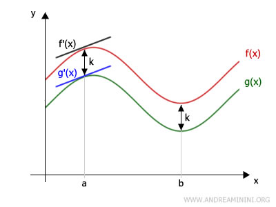
Proof. Define the auxiliary function $ z(x) $ as the difference between the two functions: $$ z(x)=f(x)-g(x) $$ Since both $ f(x) $ and $ g(x) $ are continuous on $ [a,b] $ and differentiable on $ (a,b) $, the function $ z(x) $ has the same properties. Its derivative is: $$ z'(x)=f'(x)-g'(x) $$ Because $ f'(x)=g'(x) $ by hypothesis, we have: $$ z'(x)=0 \qquad \forall \ x \in (a,b) $$ By the corollary of the Mean Value Theorem, any function that is continuous on $ [a,b] $, differentiable on $ (a,b) $, and has derivative zero throughout $ (a,b) $ must be constant on $ [a,b] $. Therefore, there exists a constant $ k $ such that: $$ z(x)=k \qquad \forall \ x \in [a,b] $$ Finally, substituting back $ z(x)=f(x)-g(x) $, we obtain: $$ f(x)-g(x)=k \qquad \forall \ x \in [a,b] $$ This completes the proof.