Quantum Electrodynamics

Quantum Electrodynamics (QED) is the quantum field theory that describes how charged particles (such as electrons, positrons, and quarks) interact with one another through the exchange of photons.

It is widely regarded as the oldest, simplest, and most successful of all quantum field theories.

QED was developed as an extension of Maxwell’s classical theory of electromagnetism, bringing it into harmony with quantum mechanics and special relativity. It also laid the groundwork for other fundamental theories, such as quantum chromodynamics and the electroweak theory.

The theory was formulated and refined in the 1940s by Tomonaga, Feynman, and Schwinger.

Why is it important? QED is extraordinarily precise: its predictions match experimental results to an accuracy of up to 12 decimal places. It also introduced some of the most powerful tools in modern physics, including Feynman diagrams and the concept of virtual particles. More broadly, QED became the prototype for all gauge theories, including the Standard Model itself.

How it works, in a nutshell

QED explains every electromagnetic interaction in terms of photon exchange between charged particles.

In other words, charged particles never act directly on one another.

The interaction occurs through the exchange of virtual photons, which appear as internal lines in Feynman diagrams.

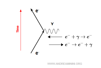
An electron may:

• emit a virtual photon  $$ e^- \;\rightarrow\; e^- + \gamma $$
• absorb a virtual photon  $$ e^- + \gamma \;\rightarrow\; e^- $$

Note. Real photons are observable particles (for example, visible light). Virtual photons, by contrast, are not free particles: they cannot be detected directly but act as intermediaries that transmit the force.

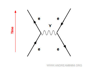
Classically, two electrons repel each other because they carry the same electric charge (Coulomb repulsion).

In QED, this repulsion is understood as a continuous exchange of virtual photons between the two electrons.

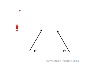
These virtual photons transfer momentum, and the exchange deflects the electrons’ trajectories, driving them apart.

This process in QED is known as Møller scattering, since it involves two electrons.

$$ e^- + e^- \rightarrow e^- + e^- $$

Thus, whenever two charged particles “sense” each other at a distance, it is not a case of instantaneous action-at-a-distance (as in classical physics), but rather the result of a quantum exchange of virtual photons.

Note. If two particles carry charges of the same sign, the exchange of virtual photons results in repulsion. If they have opposite charges, the exchange leads to attraction. Virtual photons are therefore the carriers of the electromagnetic force, capable of mediating both repulsion and attraction depending on the charges involved. This is important to stress, since it is often wrongly assumed that they “only transmit repulsion.”

Examples

Here are some of the key processes described by QED:

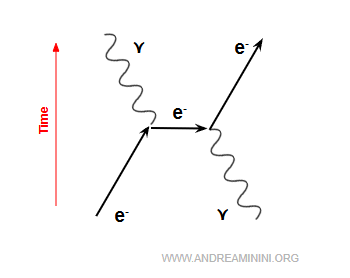
1] Compton scattering

An electron collides with a real photon and scatters it.

$$ e^- + \gamma \;\longrightarrow\; e^- + \gamma $$

In this process, a photon strikes an electron and emerges with a different wavelength (Compton effect).

It provided one of the clearest demonstrations of the particle-like nature of light.

Here is its representation in a Feynman diagram, with time flowing upward.

2] Annihilation

In this process, an electron ($e^-$) and a positron ($e^+$, its antiparticle) meet and convert their mass into energy in the form of photons.

$$ e^- + e^+ \;\;\longrightarrow\;\; \gamma + \gamma $$

Conservation of energy and momentum requires at least two photons in the final state, emitted in opposite directions.

Since photons are their own antiparticles, producing two ensures that all conservation laws are satisfied.

Here is how electron - positron annihilation appears in a Feynman diagram.

The arrow pointing opposite to the time direction represents the electron’s antiparticle, the positron.

In essence, electron - positron annihilation is the reverse of pair production ($\gamma + \gamma \to e^- + e^+$).

3] Pair production

This is the inverse of annihilation: a high-energy photon is converted into a particle - antiparticle pair, typically an electron and a positron:

$$ \gamma + \gamma  \;\;\longrightarrow\;\; e^- + e^+ $$

Two photons transform into an electron - positron pair.

In other words, pair production is the conversion of photon energy into matter (a particle and its antiparticle).

 

It is the inverse of annihilation and a striking illustration of the mass - energy equivalence, $E = mc^2$.

Note. This process cannot occur in empty space: a single photon cannot turn into a pair by itself, as that would violate momentum conservation. A nearby nucleus (or, more rarely, another electron) is required to act as a “target” and absorb some of the momentum. The real process is therefore: $$ \gamma + N \;\; \longrightarrow\;\; e^- + e^+ + N $$ where $N$ is the nucleus, which remains almost unchanged. For instance, a gamma photon striking a heavy atom can produce an $e^- + e^+$ pair.

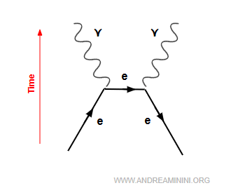
4] Bhabha scattering

This is the elastic scattering between an electron and a positron.

$$ e^- + e^+ \;\;\longrightarrow\;\; e^- + e^+ $$

It is named after Indian physicist Homi Jehangir Bhabha, who in 1935 was the first to calculate its cross section within QED.

An electron and a positron annihilate into a virtual photon.

$$ e^+ + e^- \rightarrow \gamma + \gamma $$

Almost immediately, the photon generates a new electron - positron pair $e^- + e^+$.

$$ \gamma + \gamma \rightarrow e^+ + e^- $$

In other words, an electron and a positron go in, and an electron and a positron come out. They’re not the same ones, of course, but since electrons are fundamentally indistinguishable, it makes no practical difference.

Note. A photon that appears as an internal line in a Feynman diagram is a virtual particle, unconstrained by the usual dispersion relation $ E = pc $. It can carry arbitrary energy and momentum, which places it “off-shell.” This is why the diagram can legitimately feature a single virtual photon without violating conservation laws at that vertex. In contrast, in the physical process an electron - positron annihilation must always yield two real photons to conserve both energy and momentum. The external lines of the diagram represent these real particles - as in Bhabha scattering, where the final state is once again an electron - positron pair.

What’s the difference between real and virtual photons?

In QED, it’s essential to draw a clear distinction between real photons and virtual photons.

• Real photons
  A real photon is a measurable quantum of the electromagnetic field. It propagates freely through space at the speed of light and satisfies the energy - momentum relation, meaning it lies “on-shell”: $$ E^2 = (pc)^2 + (mc^2)^2 \quad \;\; \text{with } m=0 \;\Rightarrow\; E = pc $$ Real photons are the quanta we can actually detect - whether as visible light, X-rays, or gamma radiation.

  For instance: sunlight reaching Earth, a coherent beam from a laser, or a gamma photon emitted in a nuclear decay. In practice, real photons are simply the quanta that constitute observable electromagnetic radiation.

• Virtual photons
  Virtual photons, by contrast, are best thought of as the “hidden carriers” of electromagnetic interactions. The exchange of virtual photons gives rise to forces such as the Coulomb attraction or repulsion between charges. However, a virtual photon is not a particle that can ever be detected in isolation: it appears only as an internal line in Feynman diagrams, representing intermediate states in interactions. Unlike real photons, it is not constrained by the relation $E = pc$. It can carry combinations of energy and momentum that no free photon could - hence it is said to be off-shell. In this sense, the phrase “virtual photon” is more a convenient shorthand, born from the Feynman diagram language, than a description of a physical particle.

  Note. It is sometimes said that virtual photons “exist only for an instant” thanks to the Heisenberg uncertainty principle: $$ \Delta E \, \Delta t \gtrsim \hbar $$ The idea is that a system can “borrow” an energy $\Delta E$ provided it “returns” it within a short interval $\Delta t$. The larger the energy discrepancy, the shorter the allowed time. This heuristic picture can help build intuition for why virtual photons can appear without obeying the rules governing real ones. But in rigorous QED, virtual photons have no independent existence: they are purely mathematical terms arising in perturbative calculations. Energy and momentum are conserved exactly at every interaction vertex - the only condition dropped between vertices is that of being a free, on-shell photon.

Screening in QED

In quantum electrodynamics (QED), the vacuum is not an empty void but a seething background of quantum fluctuations. For the briefest instant, these fluctuations can give rise to virtual electron - positron pairs, depicted in Feynman diagrams as a fermion loop attached to a virtual photon line. 

In this sense, the vacuum behaves much like a dielectric medium. The effect is known as vacuum polarization.

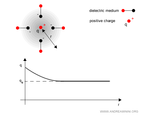
A real electric charge (say, an electron) interacts continuously with these virtual pairs.

Virtual positrons (positive charges) are pulled toward the electron’s negative charge, while virtual electrons (negative charges) are pushed outward.

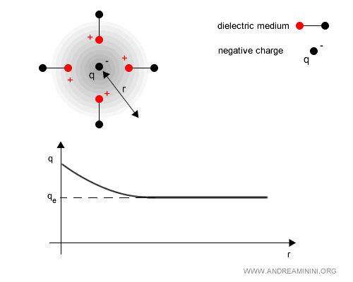
The result is a surrounding “cloud” of opposite charge that diminishes the strength of the external electric field.

At large distances, the effective charge $ q_e $ appears smaller than the bare charge $ q $.

This phenomenon is called vacuum screening.

At very short distances, however - equivalently, at high energies - one probes inside the polarization cloud and detects a larger effective charge.

This is why the electron - photon coupling constant $ \alpha $ is not a fixed quantity but depends on the energy scale, an effect known as the running of the coupling constant.

Note. The same mechanism applies to positive charges: virtual electrons cluster closer, while virtual positrons are driven away. The outcome is still vacuum polarization. 

 

Because the bare charge is always “screened,” it can only be revealed at very short distances. 

Thus, the charge we normally measure with our instruments is the “effective,” or screened, charge.

And so on.